DDIA-v2 Chinese edition: https://github.com/Vonng/ddia/tree/v2
After finishing DDIA-v2, I couldn’t put it down. Everything data-related is explained with such clarity — why is it like this? What’s the current state? What problems does this have? The observations and ideas are incredibly incisive and concise. Even the nautical-chart-style diagrams at the start of each chapter are fascinating.
Note: This article is essentially a collection of excerpts from the original work, with almost none of my own thoughts or ideas. I’ve simply plucked out the parts I love most. Some knowledge I’ve already mastered and some topics too remote are skipped!
Ch1: Trade-offs in Data System Architecture#
OLTP & OLAP#
The distinction between OLTP and analytics is not always clear-cut, but the following table lists some typical characteristics:
| Attribute | Transactional Systems (OLTP) | Analytical Systems (OLAP) |
|---|---|---|
| Primary read pattern | Point queries (fetch individual records by key) | Aggregation over a large number of records |
| Primary write pattern | Create, update, and delete individual records | Bulk import (ETL) or event stream |
| Human user example | End users of web/mobile applications | Internal analysts, for decision support |
| Machine use example | Check whether an action is authorized | Detect fraud/abuse patterns |
| Query type | Fixed set of queries, predefined by the application | Analysts can issue arbitrary queries |
| Data representation | Latest state of data (current point in time) | History of events over time |
| Dataset size | GB, TB | TB, PB |
A data warehouse is a separate database where analysts can query freely without affecting OLTP operations. Data warehouses typically store data in a very different way from OLTP databases, optimized for the query types common in analytics. The process of getting data into the data warehouse is called Extract–Transform–Load (ETL). Some database systems offer Hybrid Transaction/Analytical Processing (HTAP), aiming to enable both OLTP and analytics in a single system without ETL from one system to another. Despite the existence of HTAP, the separation between transactional and analytical systems remains common due to their differing goals and requirements. In particular, it is considered good practice for each business system to have its own database, resulting in hundreds of independent operational databases; on the other hand, an enterprise typically has only one data warehouse, allowing business analysts to combine data from several business systems in a single query. A data lake is a centralized data repository that holds any data potentially useful for analysis, sourced from business systems through ETL processes. Unlike a data warehouse, a data lake contains only files and imposes no specific file format or data model. Data warehouses typically use the relational data model and are queried via SQL. A data lakehouse goes beyond a standalone data warehouse by enabling typical data warehouse workloads (SQL queries and business analytics) as well as data science/machine learning workloads to run directly on files in the data lake. This architecture is called a data lakehouse. It requires a query execution engine and a metadata (e.g., schema management) layer to extend the file storage of the data lake. Apache Hive, Spark SQL, Presto, and Trino are examples of this approach.
Cloud Services vs. Self-Hosting#
The pros and cons of cloud services: Using cloud services, rather than running comparable software yourself, is essentially outsourcing the operation of that software to a cloud provider. There are strong arguments both for and against using cloud services.
Advantages:
- When you use the cloud, you still need an operations team, but outsourcing basic system administration can free your team to focus on higher-level problems.
- Cloud services are especially valuable if your system load varies significantly over time. If you provision machines to handle peak load but those computing resources sit idle most of the time, your system becomes less cost-effective.
- Compared to physical machines, cloud instances can be provisioned faster and come in a wider variety of sizes.
Disadvantages:
- The biggest drawback of cloud services is that you have no control over them.
- If you already have experience setting up and operating the required systems and your load is fairly predictable (i.e., the number of machines you need won’t fluctuate dramatically), it is typically cheaper to buy your own machines and run the software yourself.
- If the service lacks a feature you need, your only option is to politely ask the vendor whether they’ll add it; you usually can’t implement it yourself.
- If the service goes down, you can only wait for it to recover.
- If you use the service in a way that triggers a bug or causes performance issues, it’s very difficult to diagnose the problem. With software you run yourself, you can obtain performance metrics and debugging information from the business system to understand its behavior, and you can inspect server logs. But with vendor-hosted services, you typically don’t have access to this internal information.
- Moreover, if the service shuts down or becomes unacceptably expensive, or if the vendor decides to change its product in a way you don’t like, you’re at their mercy — continuing to run an old version of the software is usually not an option, so you’ll be forced to migrate to another service. This risk can be mitigated if there are alternative services offering compatible APIs, but for many cloud services, there is no standard API, which increases switching costs and makes vendor lock-in a real problem.
- Latency-critical applications such as high-frequency trading require complete control over hardware, making the cloud a poor choice for such businesses.
Cloud-Native#
| Category | Self-Hosted Systems | Cloud-Native Systems |
|---|---|---|
| Transactional/OLTP | MySQL, PostgreSQL, MongoDB | AWS Aurora, Azure SQL DB Hyperscale, Google Cloud Spanner |
| Analytical/OLAP | Teradata, ClickHouse, Spark | Snowflake, Google BigQuery, Azure Synapse Analytics |
The key idea behind cloud-native services is not only to use computing resources managed by the business system but also to build on top of lower-level cloud services to create higher-level services. For example:
- Object storage services like Amazon S3, Azure Blob Storage, and Cloudflare R2 store large files. They provide a more limited API than a typical filesystem (basic file reads and writes), but their advantage is hiding the underlying physical machines: the service automatically distributes data across many machines, so you don’t need to worry about running out of disk space on any single machine. Even if some machines or their disks fail entirely, no data is lost.
- Many other services are in turn built on top of object storage and other cloud services: for example, Snowflake is a cloud-based analytical database (data warehouse) that relies on S3 for data storage, and some services are further built on top of Snowflake.
Cloud-native systems are typically multi-tenant, meaning they don’t provision separate machines for each customer. Instead, data and computation from several different customers are handled by the same service on shared hardware. Multi-tenancy enables better hardware utilization, easier scalability, and simpler management for cloud providers.
Operations in the Cloud Era#
Traditionally, the people managing an organization’s server-side data infrastructure were called database administrators (DBAs) or system administrators (sysadmins). In recent years, many organizations have attempted to integrate software development and operations roles into a single team jointly responsible for backend services and data infrastructure; the DevOps philosophy has guided this trend. Site Reliability Engineers (SREs) represent Google’s implementation of this philosophy.
The DevOps/SRE philosophy emphasizes:
- Automation — preferring repeatable processes over one-off manual tasks,
- Preferring ephemeral virtual machines and services over long-running servers,
- Promoting frequent application updates,
- Learning from incidents,
- Preserving organizational knowledge about systems even as individual personnel come and go.
The operations team at an infrastructure company focuses on the details of reliably delivering services to a large number of customers, while the customers of the service spend as little time and energy on infrastructure as possible. Beyond the traditional need for capacity planning, adopting cloud services may be easier and faster than running your own infrastructure. While the cloud is changing the role of operations, the need for operations remains urgent.
Ch2: Defining Non-Functional Requirements#
Hardware and Software Faults#
In large-scale systems, hardware faults happen frequently enough that they become part of normal system operation:
- About 2-5% of disk hard drives fail each year; in a storage cluster with 10,000 disks, we can therefore expect on average one disk failure per day.
- About 0.5-1% of solid-state drives (SSDs) fail each year. Uncorrectable errors occur about once per drive per year.
- About one in 1,000 machines has a CPU core that occasionally computes incorrect results.
- Data in RAM can also be corrupted, due to random events like cosmic rays or permanent physical defects. Additionally, certain pathological memory access patterns can flip bits with high probability.
- Other hardware components such as power supplies, RAID controllers, and memory modules also fail.
- An entire data center can become unavailable (e.g., due to power outages or network misconfiguration) or even permanently destroyed (e.g., fire or flood).
Software faults are often unpredictable and, because they are correlated across nodes, can cause more system failures than hardware faults:
- A bug that causes all application server instances to crash upon receiving a specific bad input. For example, the leap second on June 30, 2012, caused many applications to hang simultaneously due to a bug in the Linux kernel.
- A runaway process that exhausts some shared resource — CPU time, memory, disk space, or network bandwidth.
- A service that the system depends on becomes slow, unresponsive, or starts returning incorrect responses.
- Cascading failures, where a small fault in one component triggers a fault in another, which triggers further faults.
Operational configuration errors are the leading cause of service outages, while hardware faults (server or network) account for only 10-25% of service outages.
Scalability Principles#
A good general principle for scalability is to decompose the system into small components that can operate relatively independently. This is the basic principle behind microservices. However, the challenge lies in knowing where to draw the line between things that belong together and things that should be separate.
If a single-machine database can do the job, it may be preferable to a complex distributed setup. A system with five services is simpler than one with fifty services. Good architecture often involves a mix of approaches.
Operations#
An operations team is critical to keeping software systems running smoothly. The typical responsibilities of a good operations team include (and go beyond) the following:
- Monitoring system health and quickly restoring service when it degrades.
- Tracking down the causes of problems, such as system failures or performance degradation.
- Keeping software and platforms up to date, including security patches.
- Understanding interactions between systems to avoid damaging changes before they cause harm.
- Anticipating future problems and addressing them before they occur (e.g., capacity planning).
- Establishing good practices for deployment, configuration, and management, and writing supporting tools.
- Performing complex maintenance tasks, such as migrating applications from one platform to another.
- Maintaining system security during configuration changes.
- Defining workflows to make operations predictable and maintain production environment stability.
- Preserving organizational knowledge about systems as personnel come and go.
Good operability means easier day-to-day work, allowing the operations team to focus on high-value tasks. Data systems can make routine tasks easier in various ways:
- Providing good monitoring with visibility into the system’s internal state and runtime behavior.
- Offering good support for automation, integrating the system with standardized tools.
- Avoiding dependence on a single machine (allowing machines to be taken down for maintenance while the overall system continues running uninterrupted).
- Providing good documentation and an easy-to-understand operational model (“if you do X, Y will happen”).
- Providing good default behavior but also allowing administrators to freely override defaults when needed.
- Self-healing when possible, but also allowing administrators to manually control system state when needed.
- Predictable behavior, minimizing surprises.
Some aspects of operations can and should be automated, but setting up correctly functioning automation in the first place still depends on humans.
Systems with too strong an individual stamp cannot succeed. When the initial design is complete and relatively stable, the real testing begins as different people test it in their own ways. — Donald Knuth
Ch3: Data Models and Query Languages#
Most applications are built by layering one data model on top of another.
- As an application developer, you observe the real world (with people, organizations, goods, actions, money flows, sensors, etc.) and model it in terms of objects or data structures and APIs that manipulate those data structures. These structures are typically specific to your application.
- When you want to store these data structures, you express them in a general-purpose data model, such as JSON or XML documents, tables in a relational database, or vertices and edges in a graph. These data models are the subject of this chapter.
- The engineers who build your database software decided on a way to represent that JSON/relational/graph data as bytes in memory, on disk, or on the network. This representation may allow the data to be queried, searched, manipulated, and processed in various ways. We’ll discuss these storage engine designs in a later chapter.
- At an even lower level, hardware engineers have figured out how to represent bytes in terms of electric currents, light pulses, magnetic fields, and so on.
SQL & NoSQL#
Databases can execute declarative queries in parallel across multiple CPU cores and machines, without you needing to worry about how to implement that parallelism. Implementing such parallel execution yourself in hand-coded algorithms would be an enormous undertaking.
The relational model, despite being half a century old, remains an important data model for many applications — especially in data warehousing and business analytics, where relational star or snowflake schemas and SQL queries are ubiquitous. However, in other domains, several alternatives to relational data have become popular:
- The document model targets use cases where data comes in the form of self-contained JSON documents and relationships between documents are rare.
- The graph data model goes in the opposite direction, targeting use cases where anything can be related to everything, and queries may need to traverse multiple hops to find data of interest (this can be expressed using recursive queries in Cypher, SPARQL, or Datalog).
- The dataframe generalizes relational data into a large number of columns, building a bridge between databases and the multidimensional arrays that form the foundation of most machine learning, statistical data analysis, and scientific computing.
Databases also tend to expand into adjacent domains by adding support for other data models: for example, relational databases have added support for document data in the form of JSON columns, document databases have added relational-like joins, and support for graph data in SQL is gradually improving.
Ch4: Storage and Indexing#
Hash Indexes#
Key-value stores are quite similar to the dictionary type found in most programming languages, which is typically implemented using a hash map or hash table.
Generally, the hash map of a hash index is kept entirely in memory. Data values can use more space than available memory because the required portion can be loaded from disk with a single disk seek.
Drawbacks of hash indexes:
- In principle, a hash map can be maintained on disk. Unfortunately, disk-based hash maps struggle to perform well. They require a large amount of random-access I/O, are expensive to grow when exhausted, and require tedious logic to resolve hash collisions.
- Range queries are inefficient. For example, you can’t easily scan all keys between kitty00000 and kitty99999 — you must look up each key individually in the hash map.
B-Tree Indexes#
B-tree indexes have been around since 1970 and are widely accepted and used in the industry. This section is familiar to most readers — skipped.
SSTables & LSM Trees#
In hash indexes, the order of key-value pairs doesn’t matter. But we can require that the sequence of key-value pairs be sorted by key. This format is called a Sorted String Table, or SSTable.
Compared to log segments using hash indexes, SSTables have several major advantages:
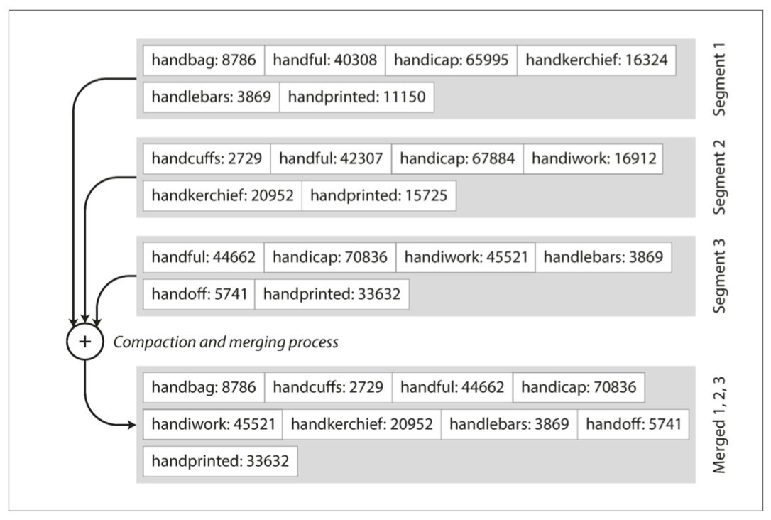
- Even if the file is larger than available memory, merging segments remains simple and efficient. The approach is like the one used in merge sort algorithms: you start reading multiple input files side by side, look at the first key in each file, copy the lowest key (according to the sort order) to the output file, and repeat. This produces a new merged segment file, also sorted by key.
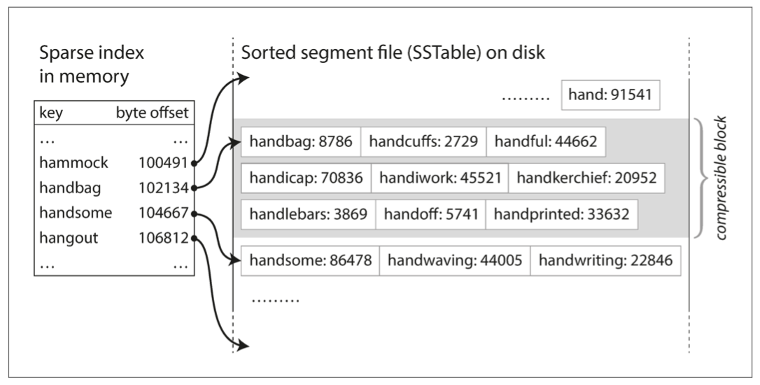
- To find a particular key in the file, you no longer need to keep an index of all keys in memory. You still need an in-memory index to tell you the offsets for some of the keys, but it can be sparse: one key per several kilobytes of segment file is sufficient, because several kilobytes can be scanned very quickly.
Using these data structures, you can insert keys in any order and read them back in sorted order. Now we can make our storage engine work as follows:
- When a new write comes in, add it to an in-memory balanced tree data structure (e.g., a red-black tree). This in-memory tree is sometimes called a memtable.
- When the memtable becomes larger than some threshold (typically a few megabytes), write it out to disk as an SSTable file. This can be done efficiently because the tree already maintains key-value pairs sorted by key. The new SSTable file becomes the most recent segment of the database. While that SSTable is being written to disk, new writes can continue on a new memtable instance.
- When a read request comes in, first try to find the key in the memtable, then in the most recent on-disk segment, then in the next older segment, and so on.
- From time to time, run a merging and compaction process in the background to combine segment files and discard overwritten or deleted values.
The algorithm described here is essentially the technique used by LevelDB and RocksDB, key-value storage engine libraries designed to be embedded in other applications. Similar storage engines are used in Cassandra and HBase, and all of them were inspired by Google’s Bigtable paper (which introduced the terms SSTable and memtable).
In-Memory Databases#
In-memory databases: As RAM becomes cheaper, the argument that RAM costs more per GB is eroding. Many datasets are not that large, so keeping them entirely in memory is quite feasible, including potentially distributed across multiple machines. This has led to the development of in-memory databases. Losing data when restarting a computer may be acceptable. Durability can also be achieved through special hardware (e.g., battery-backed RAM), by writing a change log to disk, by periodically writing snapshots to disk, or by replicating the in-memory state to other machines.
The typical in-memory database Redis provides weak durability through asynchronous writes to disk. Other in-memory databases include Memcached, VoltDB, MemSQL, Oracle TimesTen, and RAMCloud.
Counterintuitively, the performance advantage of in-memory databases does not come from avoiding disk reads. Instead, they are faster because they avoid the overhead of encoding in-memory data structures into on-disk data structures.
Materialized Views and OLAP#
Think of SQL functions like COUNT, SUM, AVG, MIN, or MAX. If the same aggregations are used by many different queries, it may be wasteful to process the raw data each time. Why not cache some of the most frequently used counts or sums? One way to create such a cache is a Materialized View.
When the underlying data changes, a materialized view needs to be updated because it is a denormalized copy of the data. The database can do this automatically, but such updates make writes more expensive, which is why materialized views are not commonly used in OLTP databases. In read-heavy data warehouses, they may make more sense because warehouses don’t have many small, frequent updates.
The advantage of a materialized data cube is that it can make certain queries extremely fast because they have already been effectively precomputed. For example, if you want to know the total sales per store, you just look at the total along the appropriate dimension without scanning millions of rows of raw data.
The disadvantage of a data cube is that it lacks the flexibility of querying raw data. For example, there is no way to compute what proportion of sales came from items costing over $100, because price is not one of the dimensions. Therefore, most data warehouses try to keep as much raw data as possible and use aggregate data (like data cubes) only as a performance boost for certain queries.
Column-Oriented Storage#
The idea behind column-oriented storage is simple: instead of storing all the values from one row together, store all the values from each column together. Column-oriented storage is easiest to understand in the relational data model, but it applies equally to non-relational data. For example, Parquet is a column-oriented storage format that supports a document data model based on Google’s Dremel.
These optimizations (column compression, sorting, etc.) make sense in data warehouses, where the workload consists mainly of large read-only queries run by analysts. Column-oriented storage, compression, and sorting all help read those queries faster. However, their drawback is that writes become more difficult.
Ch5: Encoding and Evolution#
REST vs. RPC#
Servers expose APIs over the network, and clients can connect to servers to make requests to those APIs. The API exposed by a server is called a service. Download data via GET requests, submit data to the server via POST requests.
When a service uses HTTP as the underlying communication protocol, it can be called a web service. There are two popular approaches to web services: REST and SOAP. REST is not a protocol but a design philosophy based on HTTP principles. APIs designed according to REST principles are called RESTful.
Remote Procedure Calls (RPC) are very different from local function calls:
- Local function calls are predictable and succeed or fail based only on parameters under your control. Network requests are unpredictable: requests or responses may be lost due to network problems, or the remote machine may be slow or unavailable.
- A local function call either returns a result, throws an exception, or never returns (because it enters an infinite loop or the process crashes). A network request has another possible outcome: it may return with no result due to a timeout.
- And so on.
REST seems to be the dominant style for public APIs, while RPC frameworks mainly focus on requests between services owned by the same organization, typically within the same data center.
Ch6: Replication#
Replication logs, failover, single-leader mode — the content is relatively straightforward. Skipped.
Multi-Leader Replication#
Multi-leader replication is often a retrofitted feature in many databases, so it frequently has subtle configuration pitfalls and often interacts unexpectedly with other database features. For example, auto-increment primary keys, triggers, and integrity constraints can all cause trouble. Therefore, multi-leader replication is often considered dangerous territory and should be avoided whenever possible.
However, multi-leader replication does have certain advantages, such as distributing write I/O, disaster recovery, and reducing network overhead in multi-region deployments (local writes), etc.
Write conflicts: The biggest problem with multi-leader replication is the potential for write conflicts, and resolving them is quite tricky. In principle, conflict detection could be made synchronous — i.e., wait for writes to be replicated to all replicas before telling the user the write succeeded. But this may defeat the purpose of multi-leader: if you want synchronous conflict detection, you might as well just use single-leader replication.
Resolving multi-leader write conflicts:
- Avoid conflicts. For example, have the application control that users only edit their own data.
- Converge to consistency:
- Last Write Wins (LWW). Write by timestamp — may result in data loss.
- Priority writes. Higher-priority writes win — may result in data loss.
- Extra code. Preserve conflict information and write custom conflict resolution code.
Real-time collaborative editing applications allow multiple people to edit a document simultaneously — Etherpad and Google Docs are mature examples. Databases are still very young in the area of multi-leader writes.
Multi-leader write conflicts in databases are mostly resolved or avoided at the application level. The following are relatively mature areas of write conflict research for reference:
- Conflict-free Replicated Data Types (CRDTs) are data structures such as sets, maps, ordered lists, and counters that can be concurrently edited by multiple users and resolve conflicts automatically in a reasonable way. Some CRDTs have been implemented in Riak 2.0.
- Mergeable Persistent Data Structures explicitly track history, similar to the Git version control system, and use three-way merge functions (whereas CRDTs use two-way merges).
- Operational Transformation (OT) is the conflict resolution algorithm behind collaborative editing applications like Etherpad and Google Docs. It is designed specifically for concurrent editing of ordered lists, such as lists of characters that make up a text document.
Ch7: Partitioning#
Range Partitioning and Hash Partitioning#
The drawback of range partitioning is that certain access patterns can lead to hot spots. If the primary key is a timestamp, partitions correspond to time ranges, and all writes will go to the same partition (i.e., today’s partition), which may become overloaded with writes while other partitions sit idle. You can use something other than the timestamp as the first part of the primary key to scatter the hot spot, but the drawback is that range queries won’t benefit.
Hash partitioning can mitigate the risk of skew and hot spots. For the purpose of partitioning, the hash function doesn’t need to be a cryptographically strong algorithm. The drawback of hash partitioning is that by partitioning by key hash, we lose a great property of key-range partitioning: the ability to efficiently execute range queries.
Hash partitioning can help reduce hot spots. But it cannot eliminate them entirely. For example, on a social media site, a celebrity user with millions of followers doing something can trigger a storm. This event can cause a large number of writes to the same key (the key might be the celebrity’s user ID or the ID of the action being commented on). Hash strategies don’t help here, because the hash of two identical IDs is still the same. If a primary key is very hot, a simple workaround is to add a random number at the beginning or end of the primary key. Just a two-digit decimal random number can scatter the primary key into 100 different primary keys, thus stored in different partitions. In any case, it’s about scattering hot spots, and you need to consider side effects such as the impact on range queries.
Ch8: Transactions#
ACID, BASE#
ACID is actually a very old definition. Due to the later discovery of many “anomalies,” a system claiming to guarantee ACID can’t actually articulate what exactly it guarantees. Whatever the case, ACID remains deeply ingrained — it represents the most fundamental principles of transactions. Conversely, systems that don’t meet the ACID criteria are sometimes called BASE, which stands for Basically Available, Soft State, and Eventual Consistency. BASE is a concept commonly mentioned in the NoSQL world.
The definition of BASE is even fuzzier than ACID. A simple, easy-to-understand, easy-to-remember theory of BASE: BASE (which means “alkali” in chemistry) is the opposite of ACID (which means “acid”).
You can think of it simply this way:
| Relational databases | Non-relational databases |
| Transactions | No transactions |
| ACID | BASE |
| SQL | NoSQL |
Atomicity and isolation within ACID are relatively easy to understand. The concept of consistency is actually quite vague and doesn’t seem closely related to the database itself. A quote in the book is very classic:
Joe Hellerstein pointed out that in Härder and Reuter’s paper, “the C in ACID” was “tossed in to make the acronym work,” and at the time, nobody cared much about consistency.
And the definition of isolation is very fuzzy. The industrial practice of serializability has also been stagnant. Transaction isolation can be described as “a mess,” but if serializability is a panacea, why does no one use it? Refer to this article: The History of Transactions and SSI
- Anomalies in non-serializable isolation levels generally only manifest under high concurrency; databases with low concurrency rarely encounter problems.
- When anomalies do occur, some applications may not notice them or may detect them but find them unimportant.
- Data may be anomalous, but the application may simply return an error and enter an anomaly-handling routine.
- Cost is too high. Not only is the development cost of serializable isolation levels high for databases, but applications also need adaptation costs for serializability. Just understanding this complex theory is no easy task.
- Higher isolation levels lose some performance. Massive rework may be thankless; applications need to choose between “high concurrency” and “no anomalies.”
- Businesses develop based on mechanisms, not rules. Businesses have somewhat adapted to the anomalies of weaker isolation levels, especially Read Committed.
Summed up in one sentence: It’s not like it’s unusable!
Pessimistic and Optimistic Transaction Models#
Two-phase locking is a so-called pessimistic concurrency control mechanism: it is based on the principle that if something might go wrong (e.g., another transaction holding a lock), it’s better to wait until the situation is safe before proceeding. It’s like a mutex used to protect data structures in multi-threaded programming.
In a sense, serial execution could be called the ultimate in pessimism: for the duration of each transaction, each transaction holds an exclusive lock on the entire database (or a partition of the database). As compensation for the pessimism, we make each transaction execute very fast, so the “lock” is only held for a short time.
In contrast, Serializable Snapshot Isolation is an optimistic concurrency control technique. In this context, optimistic means that if there is potential danger, the transaction is not blocked — instead, it continues executing, hoping everything will turn out fine. When a transaction wants to commit, the database checks whether anything bad happened (i.e., whether isolation was violated); if so, the transaction is aborted and must be retried. Only serializable transactions are allowed to commit. If there is a lot of contention (i.e., many transactions trying to access the same objects), performance suffers because a large proportion of transactions need to be aborted. If the system is already near maximum throughput, the additional load from retried transactions can worsen performance.
Ch9: Distributed Systems#
Clocks#
Clocks are critically important in distributed systems — they can directly affect the visibility, isolation, and correctness of transactions. In reality, reading a precise point in time is meaningless (from a quantum theory perspective, there is no concept of an absolute point in time; the actual situation is even more complex). Spanner’s Google TrueTime API reports a confidence interval for the local clock. The confidence interval reports an extremely short and trustworthy time range rather than a time point. For example, if you have two confidence intervals, each containing the earliest and latest possible timestamps ($A = [A_{earliest}, A_{latest}]$, $B=[B_{earliest}, B_{latest}]$), and these two intervals do not overlap (i.e., $A_{earliest} < A_{latest} < B_{earliest} < B_{latest}$), then B definitely happened after A — there is no doubt. Only when the intervals overlap are we uncertain about the order in which A and B occurred. To ensure that transaction timestamps reflect causality, Spanner deliberately waits for the length of the confidence interval before committing a read-write transaction. To keep the clock uncertainty as small as possible, Google deploys a GPS receiver or atomic clock in every data center, allowing clocks to be synchronized to within about 7 milliseconds. Logical clocks are based on incrementing counters rather than oscillating quartz crystals. Logical clocks only measure the relative ordering of events.
Real time may not exist. Responsiveness trumps everything. For most server-side data processing systems, real-time guarantees are uneconomical or unsuitable. Therefore, these systems must endure pauses and clock instability in non-real-time environments.
Ch10: Consistency and Consensus#
All the problems we’ve assumed are possible: packets in the network can be lost, reordered, duplicated, or arbitrarily delayed; clocks are at best approximate; and nodes can pause (e.g., due to garbage collection) or crash at any time.
CAP#
The formal definition of the CAP theorem is limited to a very narrow scope — it only considers one consistency model (linearizability) and one type of fault (network partitions, or nodes that are alive but disconnected from each other). It doesn’t discuss anything about network delays, dead nodes, or other trade-offs. Therefore, despite CAP’s historical influence, it has no practical value for designing systems.
Distributed Transactions and Consensus#
All the consensus protocols discussed so far internally use a leader in some form, but they don’t guarantee that the leader is unique. Instead, they make a weaker guarantee: the protocol defines an epoch number (called ballot number in Paxos, view number in Viewstamped Replication, and term number in Raft) and ensures that within each epoch, the leader is unique. Whenever the current leader is thought to be dead, a vote begins among the nodes to elect a new leader. This election is assigned an incrementing epoch number, so epoch numbers are totally ordered and monotonically increasing. If there is a conflict between leaders from two different epochs (perhaps because the previous leader hadn’t actually died), the leader with the higher epoch number prevails. Designing algorithms that robustly cope with unreliable networks remains an open research problem.
Ch11: Batch Processing#
Services (online systems) Services wait for requests or instructions from clients to arrive. Upon receiving one, the service attempts to process it as quickly as possible and sends back a response. Response time is typically the primary performance metric for services, and availability is usually very important (if clients can’t reach the service, users may receive error messages).
Batch processing systems (offline systems) A batch processing system takes a large amount of input data, runs a job to process it, and produces some output data. This often takes a while (from minutes to days), so typically no user is waiting for the job to finish. Instead, batch jobs typically run periodically (e.g., once a day). The primary performance metric for batch jobs is typically throughput (the time needed to process input of a certain size). This chapter discusses batch processing.
Stream processing systems (near-real-time systems) Stream processing sits between online and offline (batch) processing, so it is sometimes called near-real-time or nearline processing. Like batch processing systems, stream processing consumes inputs and produces outputs (without needing to respond to requests). However, stream jobs operate on events shortly after they occur, whereas batch jobs wait for a fixed set of input data. This difference gives stream processing systems lower latency compared to batch processing systems.
The batch processing algorithm MapReduce, published in 2004, was (perhaps over-enthusiastically) called “the algorithm that made Google’s massive scalability possible.” MapReduce is a fairly low-level programming model.
MapReduce and Distributed File Systems#
Compared to the query optimizer of a relational database, Unix tools, despite their simplicity, are still remarkably useful. The biggest limitation of Unix tools is that they can only run on a single machine — this is where tools like Hadoop came in. MapReduce is somewhat like Unix tools but distributed across thousands of machines. Like Unix tools, it’s fairly crude but surprisingly effective. MapReduce jobs read and write files on a distributed file system. In Hadoop’s implementation of MapReduce, this file system is called HDFS (Hadoop Distributed File System), an open-source implementation of the Google File System (GFS). Besides HDFS, there are various other distributed file systems such as GlusterFS and the Quantcast File System (QFS). Object storage services like Amazon S3, Azure Blob Storage, and OpenStack Swift are similar in many ways.
To create a MapReduce job, you need to implement two callback functions, Mapper and Reducer, which behave as follows:
Mapper The Mapper is called once on each input record. Its job is to extract key-value pairs from the input record. For each input, it can generate any number of key-value pairs (including none). It does not retain any state from one input record to the next, so each record is processed independently.
Reducer The MapReduce framework takes the key-value pairs produced by the Mapper, collects all values belonging to the same key, and iteratively calls the Reducer over this set of values. The Reducer can produce output records (e.g., the count of occurrences of the same URL).
Using the MapReduce programming model, the physical network communication aspects of computation (getting data from the right machines) are separated from the application logic (processing the data after obtaining it). This separation contrasts sharply with the typical use of databases, where requests to fetch data from the database frequently appear within application code. Because MapReduce handles all network communication, it also frees application code from worrying about partial failures, such as the crash of another node: MapReduce can transparently retry failed tasks without affecting application logic.
Another common pattern of “putting related data together” is grouping records by some key (like the GROUP BY clause in SQL). The simplest way to implement this grouping operation with MapReduce is to set up the Mapper so that the key-value pairs it generates use the desired grouping key. The partitioning and sorting process then directs all records with the same partition key to the same Reducer.
Hadoop vs. Distributed Databases#
As we’ve seen, Hadoop is somewhat like a distributed version of Unix, where HDFS is the file system and MapReduce is a peculiar implementation of Unix processes (always running the sort utility between the Map and Reduce phases). We’ve seen how various join and grouping operations can be implemented on top of these primitives.
When the MapReduce paper was published, it was — in a sense — not new. All the processing and parallel join algorithms we discussed in earlier sections had already been implemented over a decade earlier in so-called massively parallel processing (MPP) databases. Examples include the Gamma database machine, Teradata, and Tandem NonStop SQL, which were pioneers in this area.
The biggest difference is that MPP databases focus on executing analytical SQL queries in parallel across a set of machines, whereas the combination of MapReduce and a distributed file system is more like a general-purpose operating system that can run arbitrary programs.
Diversity of Processing Models#
Having only two processing models, SQL and MapReduce, is not enough — more diverse models are needed! And due to the openness of the Hadoop platform, implementing a whole range of approaches is feasible, something that was impossible within the monolithic MPP database paradigm. Traditionally, MPP databases met the needs of business intelligence analytics and business reporting, but this is only one of many domains that use batch processing. In the years since MapReduce became popular, execution engines for distributed batch processing have matured significantly.
Ch12: Stream Processing#
Skipped.
Event Sourcing#
Event sourcing is a powerful data modeling technique: from the application’s perspective, it’s more meaningful to record user actions as immutable events rather than recording the effects of those actions in a mutable database. Event sourcing is similar to the chronicle data model. Like change data capture, event sourcing involves storing all changes to application state as a log of change events. Applications using event sourcing need to pull the event log (representing the data written to the system) and transform it into application state suitable for display to users. The current state is derived from the event log.
Ch13: The Future of Data Systems#
Lambda Architecture#
If batch processing is used to reprocess historical data and stream processing is used for recent updates, how do we combine the two? The Lambda Architecture is one proposal for this. The core idea of the Lambda Architecture is to record incoming data by appending immutable events to an ever-growing dataset, similar to event sourcing. In the Lambda approach, the stream processor consumes events and quickly produces an approximate update to the view; the batch processor later uses the same set of events and produces a corrected version of the derived view.
Unix evolved pipelines and files that are just byte sequences, while databases evolved SQL and transactions. Which approach is better? Of course, it depends on what you want. Unix is “simple” because it’s a fairly thin wrapper around hardware resources; relational databases are “simpler” because a short declarative query can leverage a lot of powerful infrastructure (query optimization, indexes, join methods, concurrency control, replication, etc.) without requiring the query author to understand the implementation details. I interpret the NoSQL movement as a desire to apply Unix-like low-level abstractions to the domain of distributed OLTP data storage.
Separation of Application Code and State#
In theory, a database could be a deployment environment for arbitrary application code, much like an operating system. In practice, however, they are poorly suited to this goal. They don’t meet the requirements of modern application development, such as dependency and package management, version control, rolling upgrades, evolvability, monitoring, metrics, calls to network services, and integration with external systems. I believe it makes sense to have some parts of the system specialized for persistent data storage and other parts specialized for running application code. The two can interact while remaining independent. The trend is to separate stateless application logic from state management (databases): don’t put application logic into the database, and don’t put persistent state into the application.
I assert that in most applications, integrity is far more important than timeliness. Violating timeliness may be confusing and annoying, but violating integrity can be catastrophic.
Problems Introduced by Algorithms#
Bias and discrimination: For example, in racially segregated areas, a person’s ZIP code, or even their IP address, is a strong indicator of race. Given this, it seems absurd to believe that an algorithm can somehow take biased data as input and produce fair and unbiased output. Yet this view often seems to lurk among advocates of data-driven decision-making — an attitude satirized as “machine learning is like money laundering for bias.” Predictive analytics systems simply extrapolate from the past; if the past was discriminatory, they codify that discrimination into rules.
Responsibility and accountability: Automated decision-making raises questions about responsibility and accountability. If a person makes a mistake, they can be held accountable, and those affected by the decision can appeal. Algorithms also make mistakes, but when they do, who is responsible?
Privacy and surveillance: Let’s do a thought experiment. Try replacing the word data with surveillance and see if common phrases still sound as nice. For example: “In our surveillance-driven organization, we collect real-time surveillance streams and store them in our surveillance warehouse. Our surveillance scientists use advanced analytics and surveillance processing to gain new insights.”
Blind faith in the supremacy of data-driven decisions is not just delusional — it’s genuinely dangerous. As data-driven decision-making becomes more prevalent, we need to figure out how to make algorithms more accountable and transparent, how to avoid reinforcing existing biases, and how to fix them when they inevitably err.
Users barely know what data they’re giving us, what data goes into the database, and how the data is retained and processed — most privacy policies are ambiguous, stringing users along without coming clean. If users don’t understand what will happen to their data, they can’t give any meaningful consent. For users who disagree with surveillance, the only truly viable alternative is simply not to use the service. But this choice isn’t truly free either: if a service is so popular that it is “considered a necessity for basic social participation by most,” then expecting people to opt out is unreasonable — using it is effectively mandatory.
Summary#
Since software and data have such an enormous impact on the world, we engineers must remember that we have a responsibility to work toward the kind of world we want: a world that respects people, that respects humanity. I hope we can work together toward that goal.