Vector Database Core Concepts#
A Bit of History#
The development history of LLM models, from Harnessing the Power of LLMs in Practice: A Survey on ChatGPT and Beyond1:
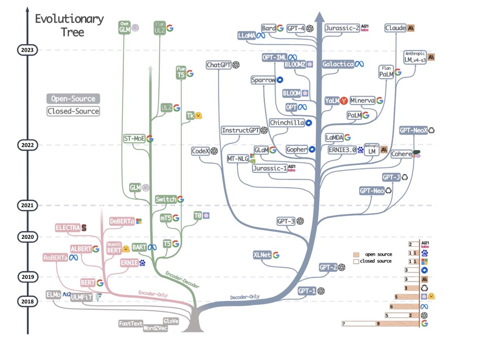
Many people only gradually learned about large models after the ChatGPT explosion, but in the years before that tipping point, the development of large models had already begun a war of the gods. Several institutions published many revolutionary papers — on the corporate side: Google, DeepMind, OpenAI, Meta, Microsoft; on the academic side: Stanford, Berkeley, CMU, Princeton, MIT2.
There are three main camps:
- Google & DeepMind camp — Gemini, Bard
- Microsoft & OpenAI camp — ChatGPT, Bing
- Meta open-source community camp — Llama
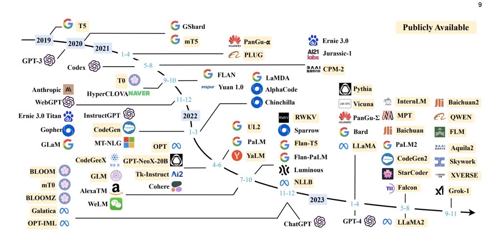
Timeline of recent large model product releases, from A Survey of Large Language Models3:
Generative AI Basics#
AIGC (Artificial Intelligence Generated Content): The precise concept of AIGC is a mode of production that uses AI to automatically generate content. In a broader sense, AIGC can be approximated as AI technology trained to possess human-like generative and creative capabilities — i.e., Generative AI. It can autonomously generate and create new text, images, music, videos, 3D interactive content, and various other forms of content and data based on data and generative algorithm models, and even includes enabling new scientific discoveries and creating new meanings.
LLM (Large Language Model): LLMs are large language models capable of capturing and processing complex language patterns and semantics — that is, they can understand and generate human language. GPT-3, ChatGPT, BERT, T5, ERNIE Bot, and others are typical large language models.
NLP (Natural Language Processing): Natural Language Processing (NLP) studies how to enable computers to read and understand human language — i.e., converting natural human language into instructions that computers can process. LLM is an important component of NLP.
AIGC has achieved remarkable growth, largely due to Natural Language Processing (NLP), and the biggest driver behind NLP’s progress is the Large Language Model (LLM). This year (2024), AIGC is also developing rapidly in areas such as video and audio.4
prompt: Instructions or directives — natural language provided to AI describing a task, used to guide a language model (such as GPT-3 or GPT-4) to generate the corresponding output5. (Everyone basically knows what this is already, no need to elaborate.)
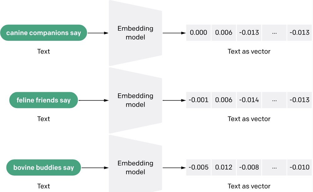
embedding:
Embedding is a method of representing objects (such as text, images, and audio) as points in a continuous vector space, where the positions of these points in space carry semantic meaning for machine learning algorithms.
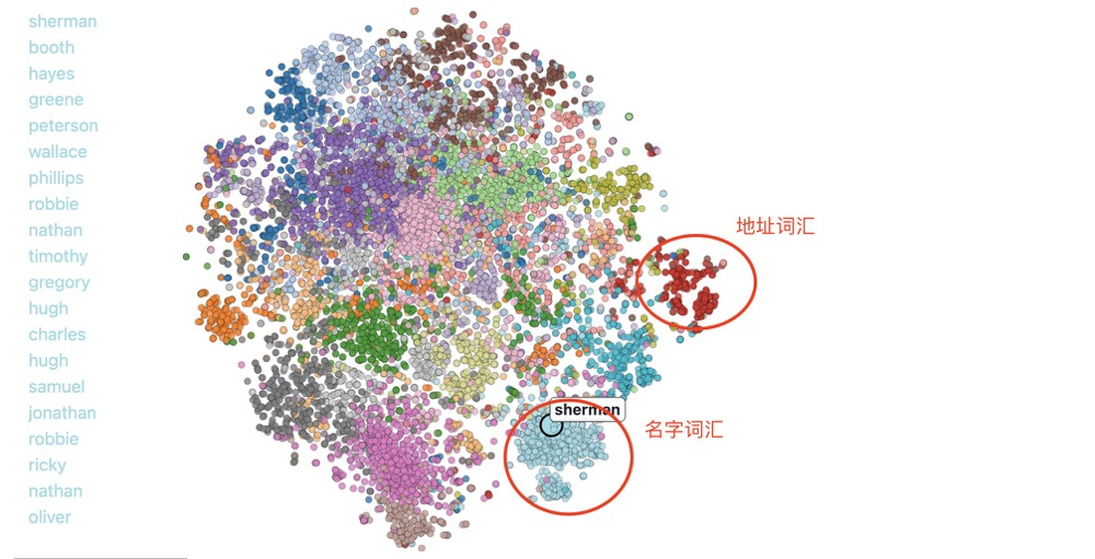
Based on GloVe word-vector relevance for English words, there is an interactive 2D embedding explorer. This shows natural language embedded as 2D vectors:
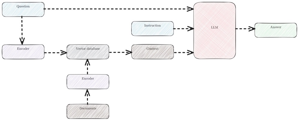
RAG#
RAG (Retrieval-Augmented Generation) is a two-stage process consisting of document retrieval and large language model (LLM) answer generation. The initial stage leverages dense embeddings to retrieve documents. Depending on the specific use case, this retrieval can be based on various database formats, such as vector databases, summary indexes, tree indexes, and key indexes5.
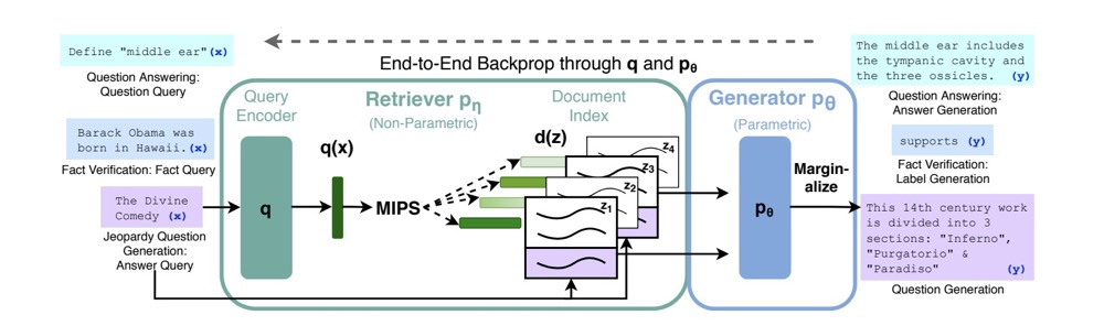
The original RAG paper6 was published on May 22, 2020, by researchers from Facebook (Meta), University College London, and New York University, proposing a general fine-tuning approach for RAG. RAG includes the following characteristics2:
- RAG models combine pre-trained memory to assist language generation
- RAG models generate language that is more specific, diverse, and factual
On March 23, 2023, OpenAI released the chatgpt-retrieval-plugin repository, recommending the use of vector databases in RAG. From that point on, vector databases gained widespread attention in the application domain, riding the wave of large model popularity.
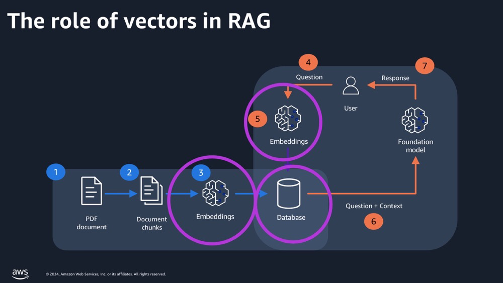
What Can Vector Databases Bring to AI?#
Vector databases can provide large models with data retrieval and long-term data storage capabilities within RAG7.
Why use RAG? No words carry more weight than those of the master, OpenAI. The following passage is from the retrieval plugin usage guide released by OpenAI in March 20238, translated by ChatGPT:
The open-source retrieval plugin enables ChatGPT to access personal or organizational information sources (with permission). Users can ask questions or express needs in natural language and obtain the most relevant document snippets from their data sources (such as files, notes, emails, or public documents).
As an open-source and self-hosted solution, developers can deploy their own version of the plugin and register it with ChatGPT. The plugin leverages OpenAI’s embeddings and allows developers to choose a vector database (such as Milvus, Pinecone, Qdrant, Redis, Weaviate, or Zilliz) to index and search documents. Information sources can be synchronized with the database using webhooks.
In short, OpenAI recommends everyone use vector databases.
Has the vector database cooled off? Not only has it not cooled off — RAG has developed to the point of being everywhere today — Has RAG Technology Really Become “Commonplace”?. And vector databases, with their high retrieval efficiency, data storage reliability, and other characteristics, are an important part of RAG.
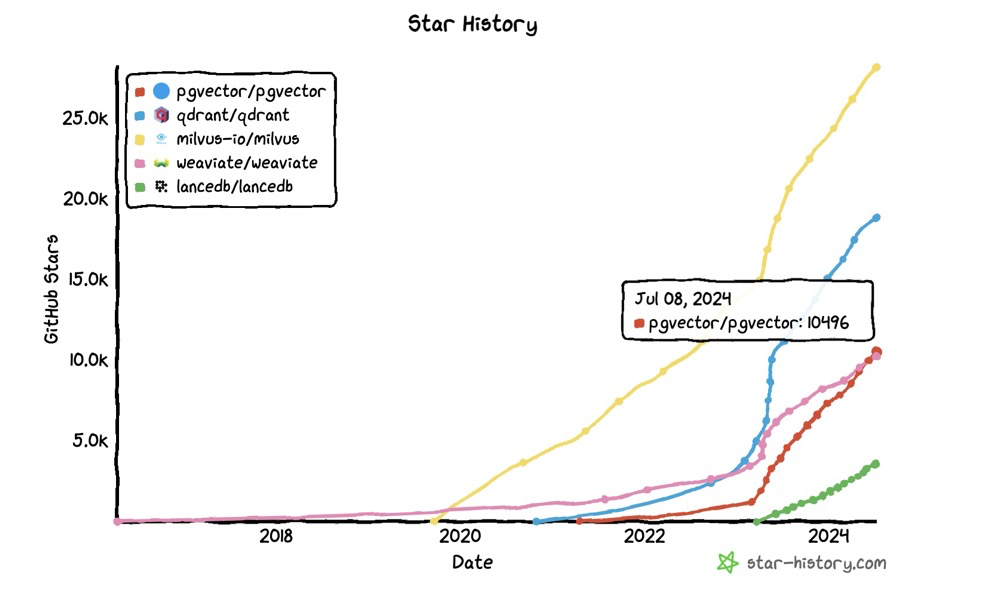
Common Vector Databases#
Since OpenAI released the RAG repo, many vector databases have emerged (though some existed before). Several companies have also secured considerable funding9:
| Company | Headquartered in | Funding |
|---|---|---|
| Weaviate | 🇳🇱 Amsterdam | $68M Series B |
| Qdrant | 🇩🇪 Berlin | $11M Seed |
| Pinecone | 🇺🇸 San Francisco | $138M Series B |
| Milvus/Zilliz | 🇨🇳 / 🇺🇸 Redwood City | $113M Series B |
| Chroma | 🇺🇸 San Francisco | $20M Seed |
| LanceDB | 🇺🇸 San Francisco | Venture |
| Vespa | 🇳🇴 / 🇺🇸 Indianapolis | Yahoo! |
| Vald | 🇯🇵 Tokyo | Yahoo! Japan |
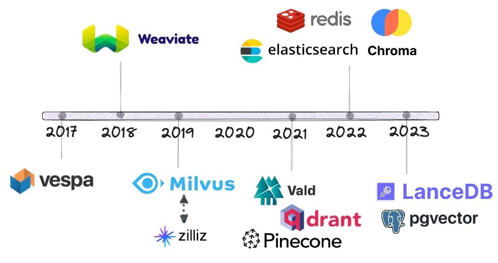
Vector database release timeline:
Vector database performance comparison10:
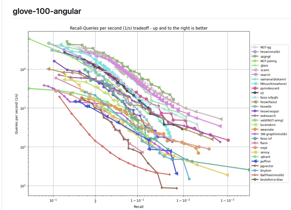
Dedicated vector databases generally perform better than traditional databases with vector plugins, for roughly two reasons:
- Dedicated vector databases are built with vector-specific underlying storage, and their performance is generally better than untargeted traditional databases.
- Dedicated vector databases are generally newer (mostly implemented in Go or Rust), making code-level optimization easier.
However, this does not mean plugin-based vector databases have no place:
- Traditional databases natively support more features, not just similarity computation.
- ACID — traditional database storage is safer.
- It’s easier to manipulate data within a single database.
Vector database feature comparison:
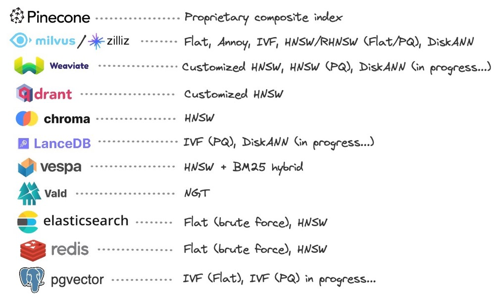
The description of pgvector above is no longer entirely accurate — pgvector now supports HNSW, and the pgvector ecosystem project pgvectorscale also supports DiskANN.
Mathematical Concepts#
Mathematics says: “I stand on the mountaintop watching you all play.”
Scalar#
A scalar is a specific number. Scalars have no direction and are generally defined in contrast to vectors.
Vector#
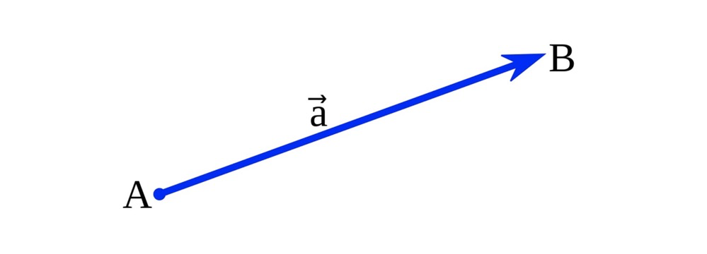
In Euclidean space, a vector has both magnitude and direction. For example, vector a from point A to point B (contains information about both points and direction)11:
Unit Vector#
A vector with magnitude one is a unit vector. The unit vector equals the vector divided by its Euclidean length12: $$ \vec a = \frac{\mathbf a}{||\mathbf a||} $$
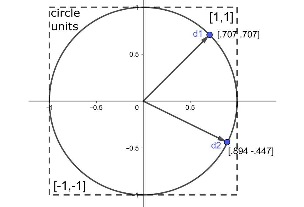
In mathematics, the Unit Vector is called a “normalized vector” in pgvector and OpenAI embeddings. (Note: do not confuse this with the mathematical concept of the normal vector — a normal vector is a different concept entirely.)
Why use unit vectors?
OpenAI embeddings’ explanation for using unit vectors13:
OpenAI embeddings are normalized to length 1, which means that:
- Cosine similarity can be computed slightly faster using just a dot product
- Cosine similarity and Euclidean distance will result in the identical rankings
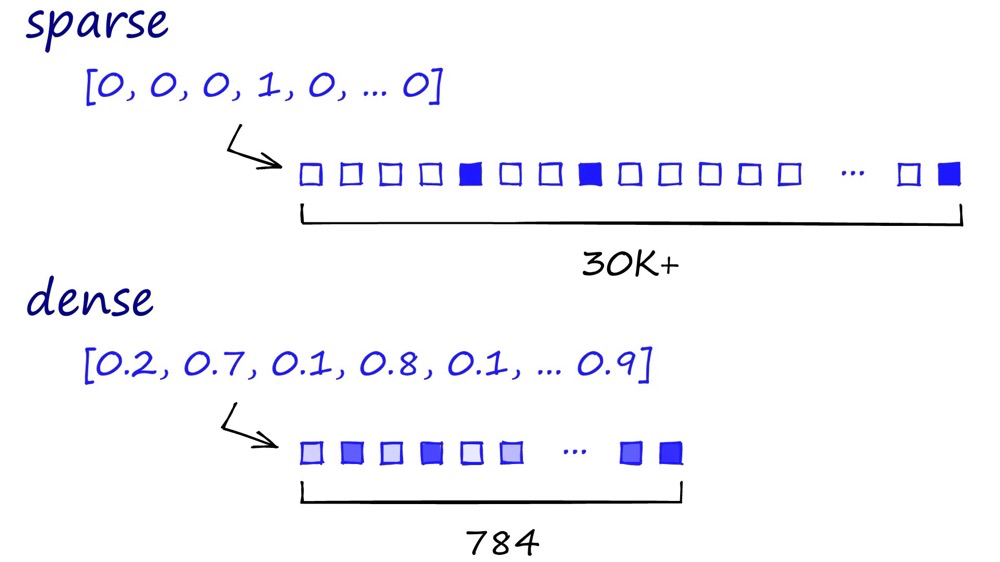
Sparse Vector#
Sparse vectors are called “sparse” because the information in the vector is sparsely distributed. Typically, we need to find a few ones (relevant information) among thousands of zeros. Therefore, these vectors can contain many dimensions, usually in the tens of thousands.
Comparison of sparse and dense vectors: Sparse vectors contain sparsely distributed bits of information, while dense vectors carry more information in every dimension — information-dense.14
Euclidean Space#
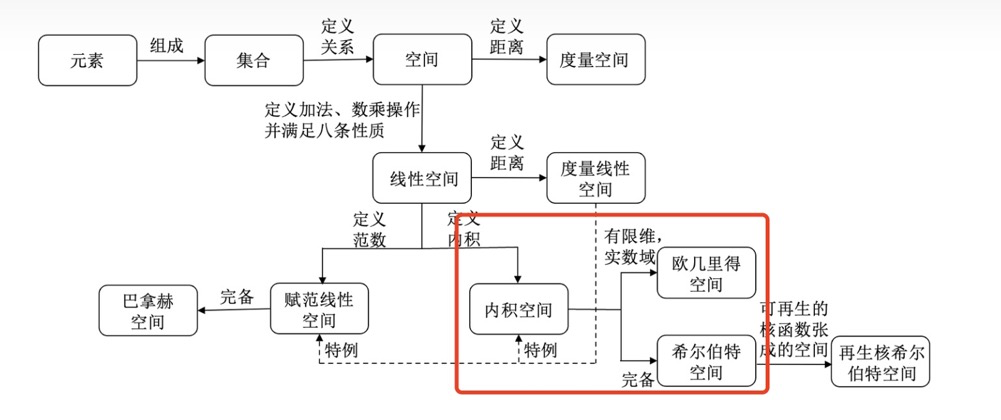
Simply called Euclidean space, it is the most fundamental space in mathematics. In modern mathematics, a space of positive integer n dimensions is called Euclidean space.
There are other space definitions, such as inner product space and Hilbert space. They differ in mathematical definitions, but in database/real-world contexts, the distinctions are not so fine-grained. The key takeaway is that inner product space, Euclidean space, and Hilbert space can all contain elements such as points, vectors, and inner products — we can simply call them “multi-dimensional spaces”. For their differences, see A Casual Discussion of Various Spaces in Mathematics15.
Euclidean Distance#
Simply called Euclidean distance, this is what we generally think of as the distance between points — i.e., the length of a line segment16.
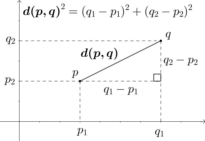
In 2D space, the Euclidean distance between points q and p is: $$ d(\mathbf p,\mathbf q)=\sqrt{(p_1-q_1)^2+(p_2-q_2)^2} $$
In n-dimensional space, the Euclidean distance between points q and p is: $$ d(\mathbf p,\mathbf q)=\sqrt{(p_1-q_1)^2+(p_2-q_2)^2+\cdots+(p_n-q_n)^2} $$
Manhattan Distance (or Taxicab Distance)#
$$ d(\mathbf p,\mathbf q)= \sum_{i=1}^n | p_i-q_i| $$
Manhattan distance is the sum of the absolute differences of two points across each dimension17.
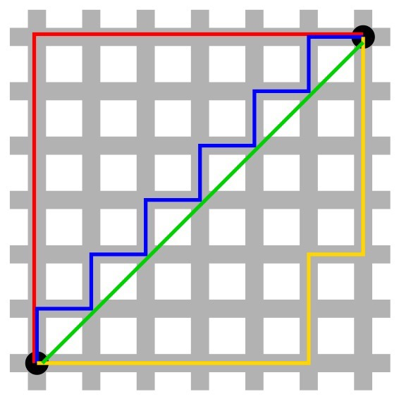
In the figure above, the green line is Euclidean distance; the red, yellow, and blue lines are Manhattan distances.
Minkowski Distance#
$$ d(\mathbf a,\mathbf b)= \left( \sum_{i=1}^n | a_i-b_i|^p \right)^{1/p} $$
The figure below shows the distance from the origin to a point of unit length at different values of p in Minkowski distance18:
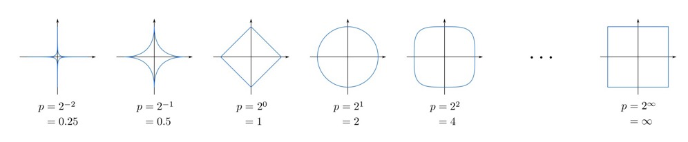
- When p=1, it is Manhattan distance, also written as “L1 distance”
- When p=2, it is Euclidean distance, also written as “L2 distance”
- When p=n, it is Minkowski distance, also written as “Ln distance”
Cosine Similarity#
The cosine value of the angle between two vectors — also called cosine similarity. Cosine similarity depends only on the angle between the two vectors, not on the vectors’ lengths19.
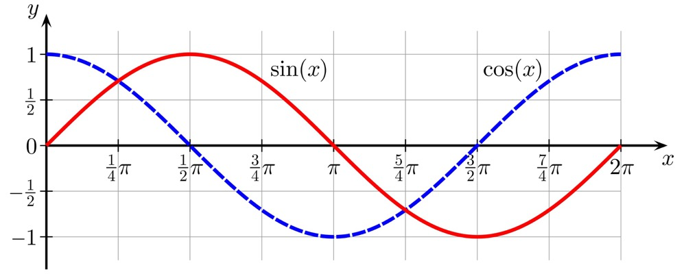
The smaller the angle between two vectors, the larger the cosine similarity. Value range: [-1, 1]. cos(0)=1, cos(90)=0, cos(180)=-1.
Cosine similarity between two vectors is written as: $$ cos (\theta) $$ Expressed in vector form: $$ cos (\theta)=\frac{\mathbf a\cdot \mathbf b }{||\mathbf a|| , ||\mathbf b||}= \frac{ \sum_{i=1}^n \mathbf a_i \mathbf b_i}{ \sqrt {\sum_{i=1}^n \mathbf a_i ^2} \cdot \sqrt {\sum_{i=1}^n \mathbf b_i ^2}} $$
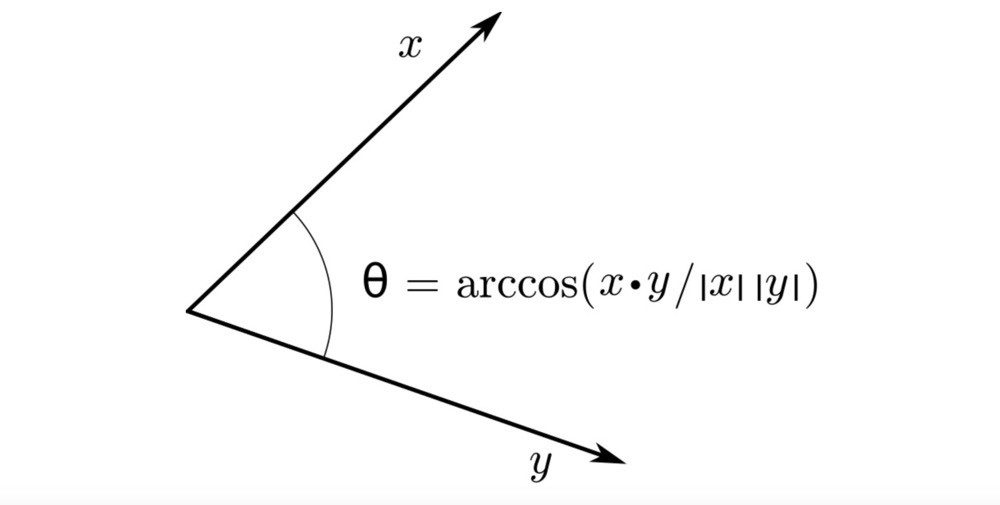
Inner Product#
Also called the dot product, it can be used to represent the length and angle of vectors. The inner product equals the Euclidean distance of the vectors multiplied by the cosine of the angle between them.
Inner product in 2D space: $$ \mathbf a\cdot \mathbf b=||\mathbf a|| , ||\mathbf b||, cos \theta $$ or $$ \mathbf a\cdot \mathbf b= a_1 b_1 + a_2 b_2 $$ Inner product in n-dimensional space (a=[a1,a2,···,an], b=[b1,b2,···,bn]): $$ \mathbf a\cdot \mathbf b=\sum_{i=1}^n a_ib_i= a_1b_1 + a_2b_2 + \cdots + a_nb_n $$
Now the following diagram should make sense. Using the formulas above, you can also reverse-engineer what the distance operators mean for n-dimensional vectors.
They are: Euclidean distance, cosine distance, and inner product20.
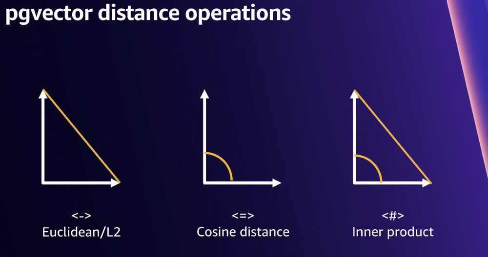
All three can describe the similarity between two vectors.
- Euclidean distance: contains only distance information between the two vectors
- Cosine distance: contains only angle information between the two vectors
- Inner product: contains both distance information and angle information
Of course, there are more mathematical models for vector similarity computation, but it depends on whether the vector database supports them.
Jaccard Distance#
In short: intersection divided by union21.
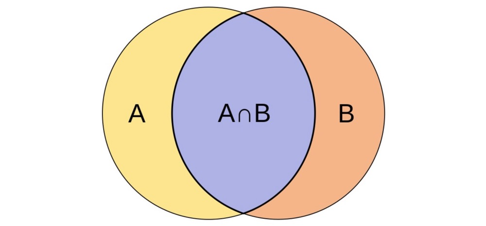
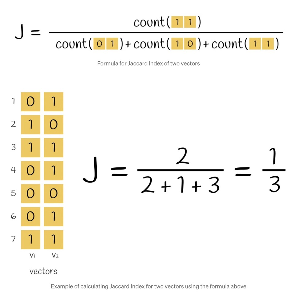
Formula: $$ J(A,B)= \frac{|A\cap B| }{|A \cup B|} $$
Expressed in vectors, it computes the ratio of the count of equal elements to the count of unequal elements22.
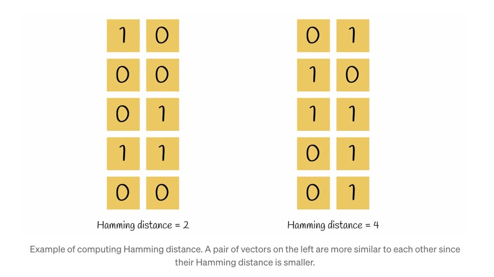
Hamming Distance#
The number of differing positions between two strings or vectors of equal length23.
Examples:
- “karolin” and “kathrin” is 3.
- “karolin” and “kerstin” is 3.
- “kathrin” and “kerstin” is 4.
- 0000 and 1111 is 4.
- 2173896 and 2233796 is 3.
Illustration24:
Delaunay Triangulation#
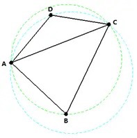
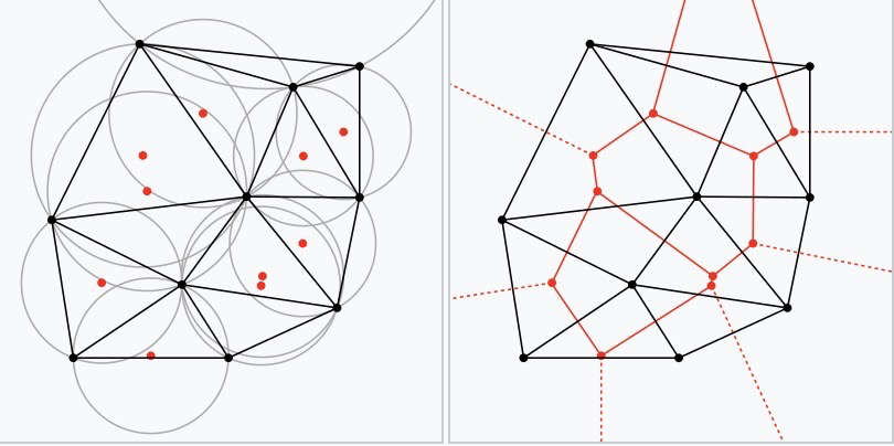
Delaunay triangulation is an operation on a set of points in a plane. It subdivides the convex hull of these points (which contains multiple points) into multiple triangles, where the circumcircle of each triangle contains no point from the set. This maximizes the minimum angle among all triangles and tends to avoid producing skinny triangles25.
Does NOT satisfy “the circumcircle of each triangle contains no point from the set”:
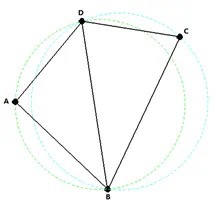
DOES satisfy “the circumcircle of each triangle contains no point from the set”:
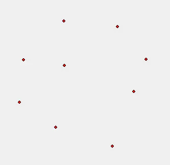
For example, triangulating a point set:
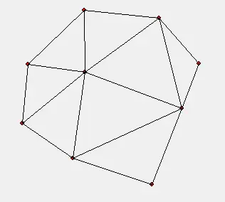
A valid triangulation:
Delaunay triangulation is not actually an algorithm — it merely defines what a “good” triangular mesh looks like. Its excellent properties are the empty-circle property and the maximized-minimum-angle property. These two properties avoid the creation of skinny triangles and make Delaunay triangulation widely applicable.
Voronoi Diagram#
Delaunay triangulation is a triangulation of a discrete point set P in general position, and it corresponds to the dual graph of P’s Voronoi diagram. The circumcenters of Delaunay triangles are the vertices of the Voronoi diagram. In 2D, Voronoi vertices are connected by edges, which can be derived from the adjacency relationships of Delaunay triangles: if two triangles share an edge in the Delaunay triangulation, their circumcenters should be connected by an edge in the Voronoi tessellation26:
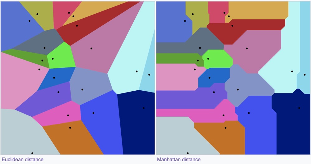
The key property of a Voronoi diagram is: the distance from a centroid to any point within its region is smaller than the distance from that point to any other centroid. $$ R_k={x \in X ,|,d(x,P_k) \le d(x,P_j) ; \mathrm{for ,all },j \neq k} $$ Rk is the centroid, d(x,Pk) is the distance from the centroid to any point within its region, and d(x,Pj) is the distance from other centroids to any point in that region.
Due to different ways of computing the distance d, Voronoi diagrams can take on different appearances27:
Vector Database Indexes#
Nearest Neighbor Search#
ENN (Exact Nearest Neighbor): Finding the point or vector closest to a query point in a given dataset. This method guarantees the highest accuracy, but as the dataset size increases, the computational cost rises sharply because it requires evaluating the distance between the query point and every point in the dataset.
ANN (Approximate Nearest Neighbor): To improve efficiency, approximately finding the nearest point to the query point at the cost of some accuracy. This method is implemented through various algorithms and can significantly reduce computational cost, especially effective when dealing with large-scale datasets.
KNN (K-Nearest Neighbors): A commonly used machine learning algorithm that works by finding the K nearest neighbors to a given query point in the dataset.
Index Evaluation Criteria#
Evaluating the quality of an index always depends on the specific data model, but in general, it includes the following points:
- Query time: Query speed is critical, especially important in large model contexts.
- Query quality: ANN queries won’t always return perfectly accurate results, but the query quality must not deviate too much. Query quality has many metrics, the most common being recall.
- Memory consumption: The memory consumed by the query index — searching in memory is clearly faster than searching on disk.
- Training time: Some search methods require training to reach a good state.
- Write time: The impact on the index when writing vectors, including all maintenance.
Most of these metrics are straightforward. Here we’ll focus on query quality:
In ANN search, results are not always exact. When searching a set of elements, the concepts include: the query scope (retrieved elements), all correct elements (relevant elements), the returned correct elements (true positives), and the returned incorrect elements (false positives)28:
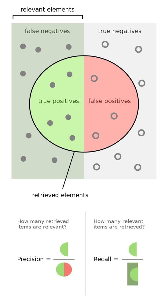
TP = True positive; FP = False positive; TN = True negative; FN = False negative
Accuracy: $$ Accuracy=\frac{TP+TN}{TP+FP+TN+FN} $$ or: $$ Accuracy=\frac{\text{all correct elements}}{\text{all elements}} $$
Precision: $$ Precision=\frac{TP}{TP+FP} $$ or: $$ Precision=\frac{\text{retrieved correct elements}}{\text{all retrieved elements}} $$
Recall: $$ Recall=\frac{TP}{TP+FN} $$ or: $$ Recall=\frac{\text{retrieved correct elements}}{\text{all correct elements}} $$
F-measure: Equivalent to weighted precision and recall $$ Recall=2 \cdot \frac{precision \cdot recall}{precision+recall} $$
Example: Consider a computer program designed to identify dogs (and related elements) in digital photos. When processing a photo containing ten cats and twelve dogs, the program identifies eight dogs. Among the eight identified as dogs, only five are actually dogs (true positives), while the other three are cats (false positives). Seven dogs were missed (false negatives), and seven cats were correctly excluded (true negatives). For this program:
- Accuracy = 12/(10+12) (largely independent of the identification program itself)
- Precision = 5/8 (true positives / all retrieved elements)
- Recall = 5/12 (true positives / all correct elements)
- F-measure = 2*[(5/18)*(5/12)]/[(5/18)+(5/12)]
Locality-Sensitive Hashing (LSH)#
LSH is a method for narrowing the search scope by converting data vectors into hash values while preserving information about their similarity.
LSH Construction#
LSH has many implementations. Here we introduce the more traditional one. This traditional LSH implementation consists of three parts22:
- Shingling: Encode the original text into vectors.
- MinHashing: Convert the vectors into a special representation called a signature, used for comparing similarity between them.
- LSH function: Hash the signatures into different buckets. If a pair of vectors’ signatures fall into the same bucket at least once, they are considered candidates.
Shingling#
Shingling is a method of embedding (in my personal opinion). Shingling identifies natural language as k consecutive tokens, with duplicate tokens removed22:
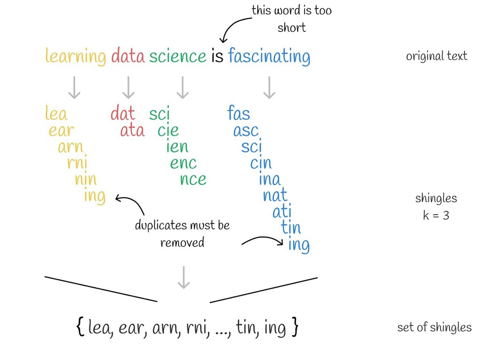
At this point, we have a set of tokens based on k-grams. The next step is to convert them into vectors.
Start with an all-zero vector, whose length equals the length of the token set. Set the position corresponding to each token to 1:
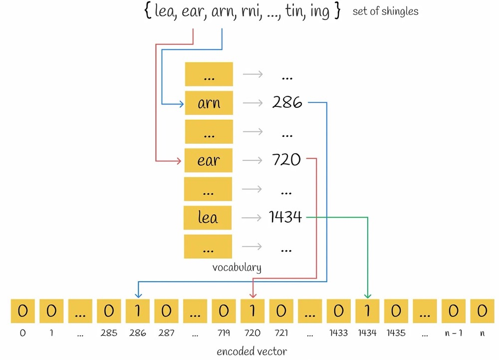
The final result is a very long vector containing only 0s and 1s, where the vector’s information captures the semantics of a sentence.
MinHashing#
Since the vector dimensionality is extremely high, directly computing approximate distances using one-hot encoded vectors yields very poor results. We need to convert sparse vectors into dense vectors — this process is called MinHashing in LSH, and the converted vector is called a MinHashing signature.
MinHashing can be a bit tricky for beginners at first, but once you grasp it, you’ll find it very simple.
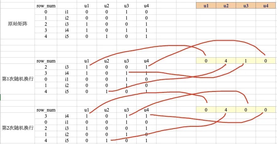
MinHashing is a hash function that permutes the components of an input vector and then returns the first index where the permuted vector component equals 1.
- First, apply a permutation: rearrange the components of a vector.
- Return the index of the first element that equals 1 after permutation.
For example:
u1 vector (0,0,1,1,0): after the first random permutation, the corresponding index is 0; after the second random permutation, the corresponding index is 029. u1’s MinHashing signature is (0,0).
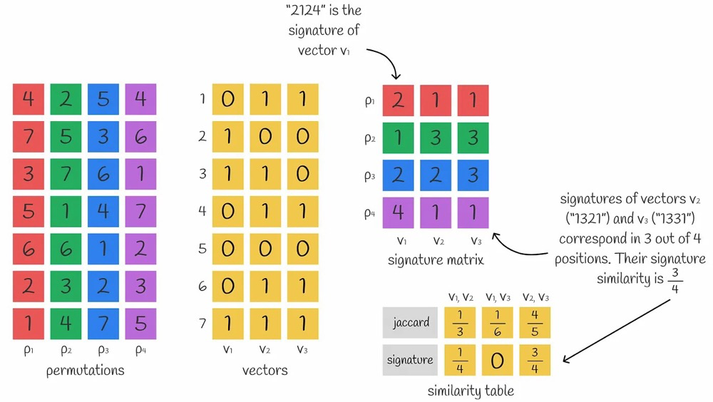
In practice, multiple minhash values can be used to approximately compute the Jaccard similarity between vectors. The more minhash values used, the more accurate the approximation.
LSH Function#
Even after converting sparse vectors into dense vectors, the dense vectors can still have high dimensionality, making direct retrieval inefficient.
We can improve query efficiency using hash tables. However, note that using a completely random hash algorithm easily places nearby vectors into different hash buckets. We need a hash algorithm that places nearby vectors into the same hash bucket — this is LSH: Locality-Sensitive Hashing.
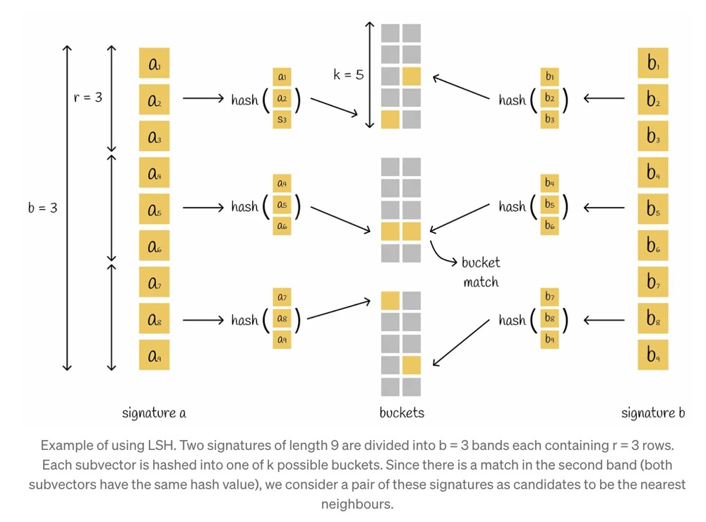
The LSH mechanism builds a hash table consisting of several parts which puts a pair of signatures into the same bucket if they have at least one corresponding part.
The concept of locality-sensitive hashing is also simple: split the signature into bands, compute hash values for each sub-signature band, and designate those with colliding sub-hash values as candidates.
The following example is easy to understand — read through it:
Thinking in terms of extremes: b=1 means no banding at all — direct hashing, completely defeating the purpose of LSH. b=number of signature elements means one band per element, i.e., one hash value per element — this can achieve relatively accurate approximate comparison, but it imposes a massive burden on computation and memory.
LSH Parameters and Error Rate#
The probability that a vector becomes a candidate vector directly affects recall. The probability of a candidate vector is as follows, where:
- s represents similarity
- b represents the number of bands
- r represents the number of rows per band
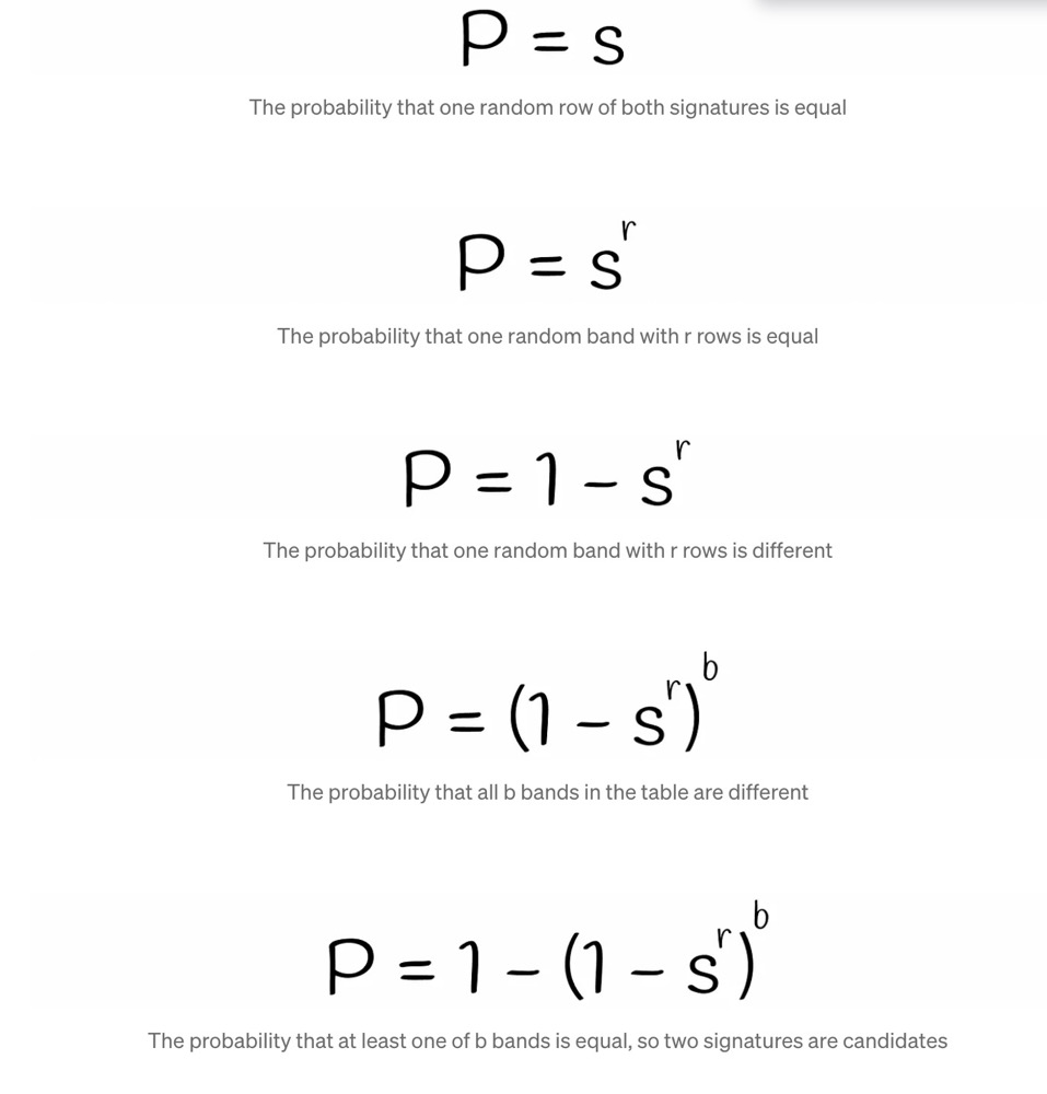
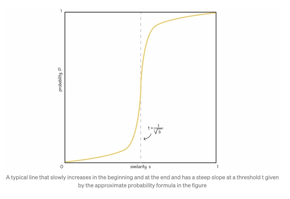
If we plot P against s using the formula, the relationship between vector similarity and candidate probability is as follows:
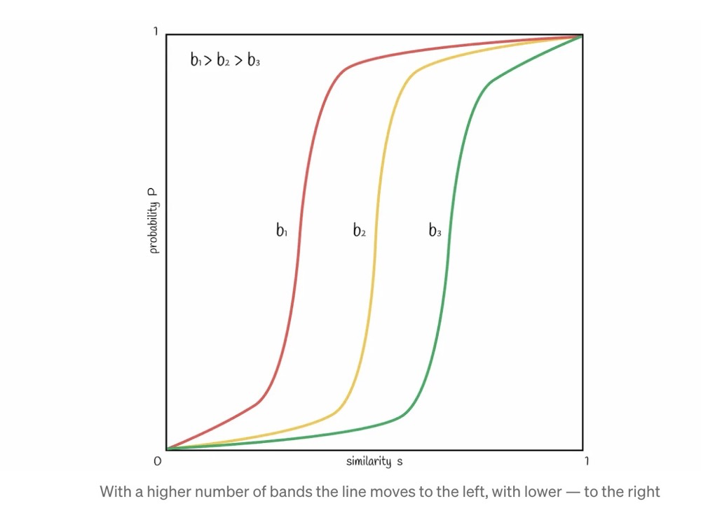
The larger the number of bands b, the smaller the candidate similarity probability.
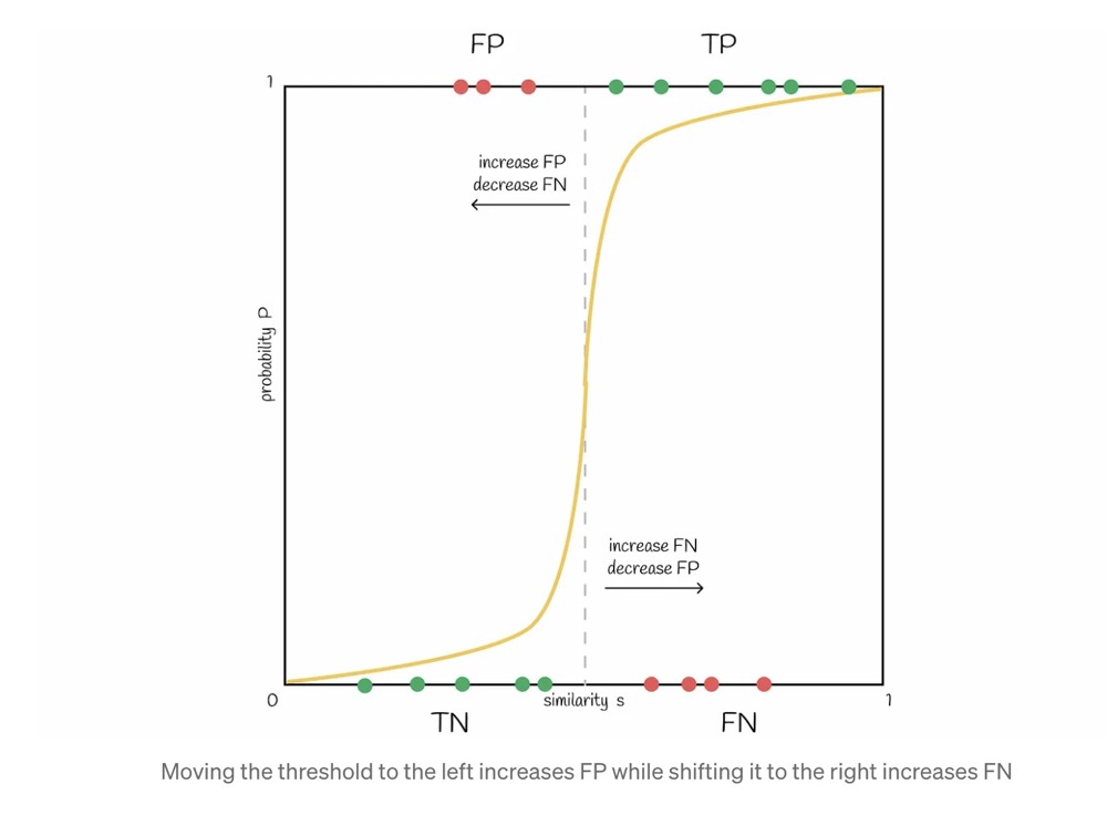
At the same time, adjusting b and s affects P, and P is related to FP and TN.
For example, returning more candidates naturally leads to more false positives — i.e., returning non-similar “candidate pairs.” This is an inevitable consequence of modifying the parameter b.
TP = True positive; FP = False positive; TN = True negative; FN = False negative
LSH is susceptible to high-dimensional data: more dimensions require longer signatures and more computation to maintain good search quality. In such cases, other indexes are recommended.
More#
There are two more articles I haven’t finished digesting — they seem to be related to binary vectors and Euclidean distance:
https://towardsdatascience.com/similarity-search-part-7-lsh-compositions-1b2ae8239aca
HNSW Index#
The HNSW algorithm (Hierarchical Navigable Small World) is a multi-layer graph-based proximity algorithm. HNSW is currently one of the most popular vector index algorithms.
At a high level, HNSW is based on the Small World Theory. The Small World Theory originally stems from the Six Degrees of Separation theory in social psychology — any two people can be connected through at most five layers of social relationships. In other words, any two people on Earth can be connected through at most six steps of social connections. The Small World Theory was later widely accepted through experimental and empirical evidence and extended to non-social relationship networks. Note that the Small World Theory is a phenomenon.
In short, the Small World Theory explains that “the connection between two entities is actually very short.” What HNSW does is establish connections between elements and reduce the number of connections.
HNSW Index Construction#
Let’s look at the HNSW paper’s algorithm for constructing HNSW graph layers30:
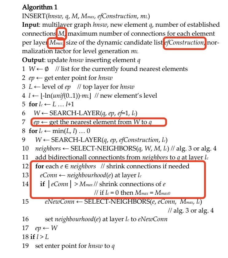
Several elements in the construction algorithm are important:
- M is the number of new edges (connections) added, representing the number of new edges for a newly inserted node.
- Mmax is the maximum number of edges per node. If neighboring nodes are inserted continuously, the edge count of existing neighboring nodes could keep increasing, wasting computational resources during search. When inserting a new node causes an existing neighboring node’s edge count to exceed Mmax, shrink connection is needed.
- efConstruction is the set of neighboring nodes.
Construction illustration31:
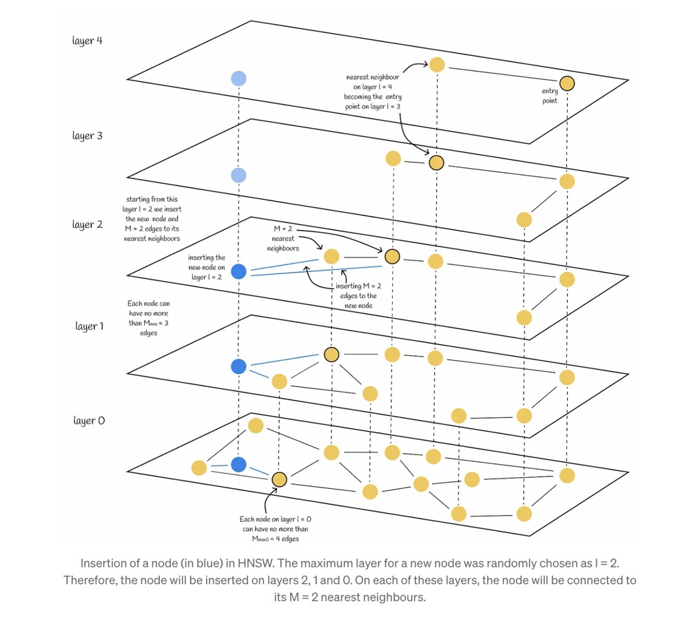
Steps for HNSW node insertion (without shrink connection):
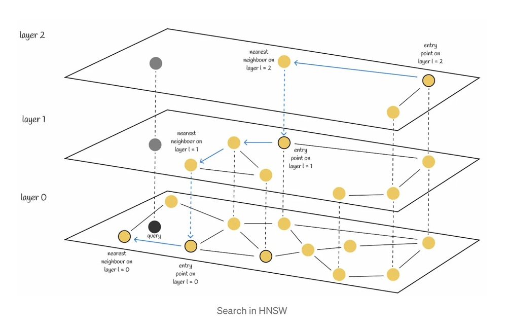
- When a new node is inserted, first find neighboring nodes at the top layer using efConstruction. Use the found nearest neighbor as the entry point to descend to the next layer, then continue searching for neighbors using that layer’s efConstruction.
- Perform node insertion at a certain layer (e.g., L=2). Select M nodes from efConstruction and connect them to the new node — at this point, 1 new node is added with M edges connected to it.
- Repeat step 2 until reaching the bottom layer (layer0).
HNSW Heuristic Neighbor Selection#
The basic HNSW index structure construction has another problem: if two clusters are relatively far apart, according to the basic HNSW construction algorithm, the two clusters are almost impossible to connect, because the basic HNSW construction algorithm is built on the nearest neighbor nodes in efConstruction.
The HNSW original paper not only proposed the basic HNSW construction algorithm but also introduced a heuristic algorithm for solving the isolated cluster problem:
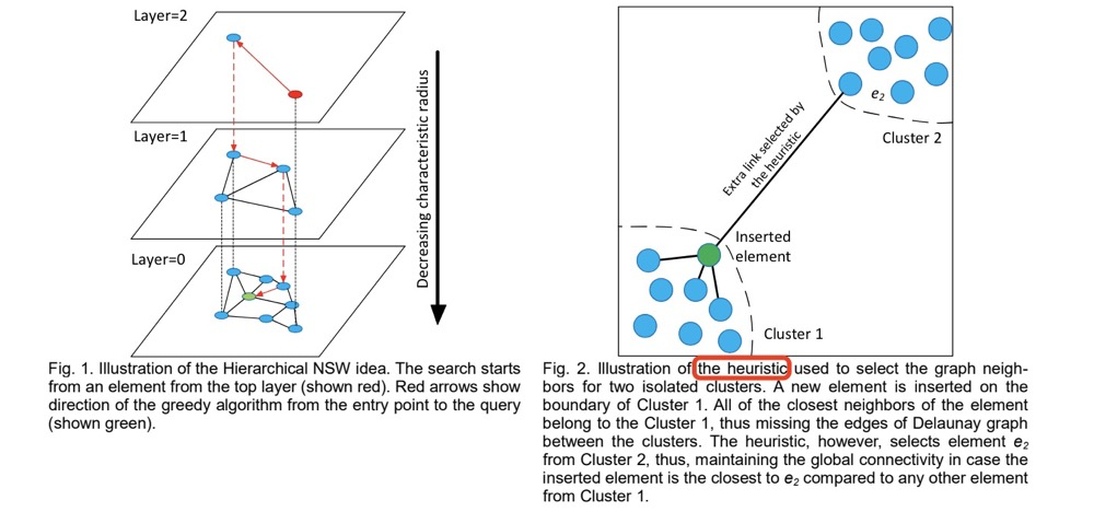
Fig.2 Heuristic for selecting graph neighbors for two isolated clusters. A new element is inserted on the boundary of cluster 1. All the element’s nearest neighbors belong to cluster 1, thus missing the Delaunay triangulation edges between the clusters. However, the heuristic selects element e2 from cluster 2, so if the inserted element is closer to e2 than to any other element from cluster 1, global connectivity is maintained.
“The heuristic algorithm not only considers the nearest distance between nodes in the graph but also considers connectivity between different regions of the graph.”
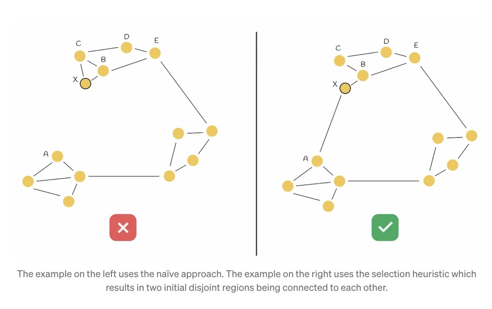
As shown below, when adding node X, the heuristic algorithm should be applied here — establishing connectivity with cluster A, rather than simply adding to the nearest neighbor nodes:
HNSW Index Search#
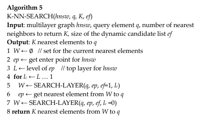
The main logic of HNSW’s KNN search method as described in the HNSW original paper consists of the following two algorithms:
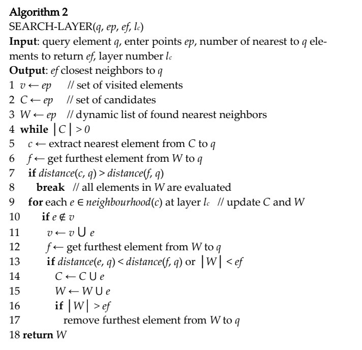
- Algorithm 2 appears slightly more complex, but the logic is actually simple — Algorithm 2 finds the set of nearest neighbor nodes ef for q at that layer. In simple terms, Algorithm 2 adds candidate nodes to the ef set, compares distances, and removes the farthest nodes, so the returned W is the ef for q at that layer.
- Algorithm 5 returns the K nearest neighbor nodes of q. It calls Algorithm 2 twice (or more). The first line in the for loop has input parameter ef=1, meaning non-bottom layers only find the single nearest ep (entry point). The bottom layer (lc=0) returns the K nearest neighbor node set W.
HNSW Complexity#
The number of HNSW layers is a function of log(N).
Search complexity: Complexity can be rigorously evaluated in a Delaunay graph, with the average complexity being O(log(N)) (for non-Delaunay graphs, such as graphs with heuristic neighbor selection, the paper does not provide a specific complexity formula).
Construction complexity: HNSW is constructed by iteratively inserting all elements, with average complexity O(N∙log(N)).
HNSW Index Parameters#
Generally, HNSW indexes for vector data have several adjustable parameters that affect index construction speed, recall, etc. Different databases may have slightly different parameters. Here we use pgvector’s HNSW parameters as an example:
Index construction parameters:
- m: Maximum number of edges per vector, default 16. Equivalent to Mmax in the paper.
- ef_construction: Number of vectors in the neighbor list during index construction, default 64. Equivalent to ef_construction in the paper.
Index search parameters:
- hnsw.ef_search: Adjusts the number of vectors in the neighbor list during search (also equivalent to ef_construction in the paper). Must be greater than or equal to limit.
Impact of adjusting ef_construction on creation time and recall during index construction20:
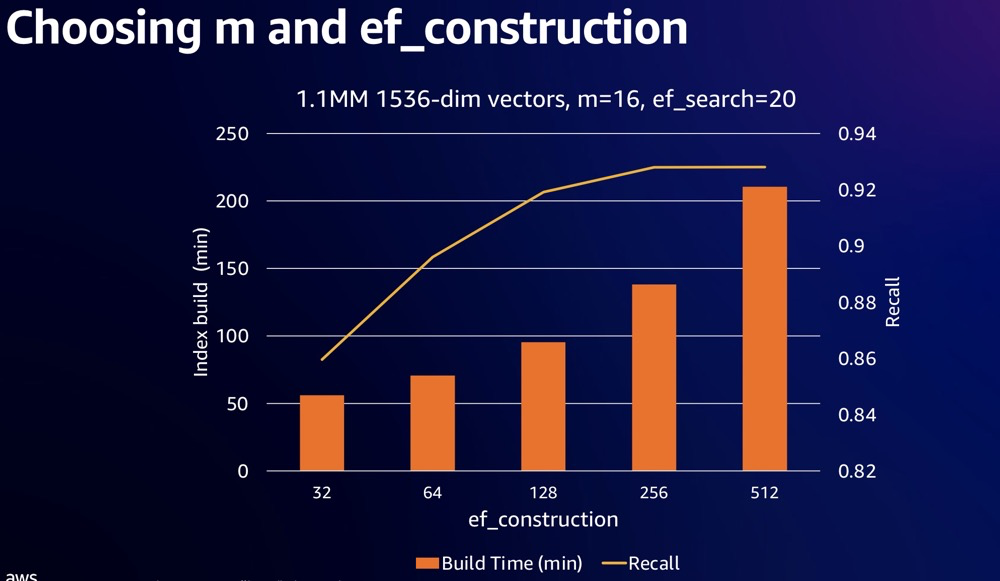
Increasing ef_construction improves recall but extends index creation time. After ef_construction=256, index construction time increases noticeably but recall improvement is not obvious.
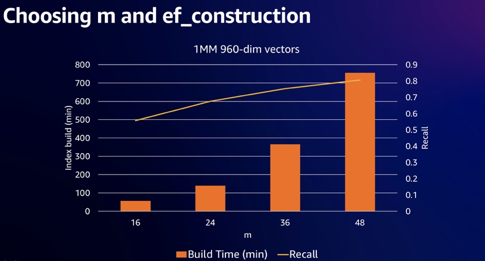
Increasing m also improves recall and extends index creation time. After m=36, index construction time increases noticeably but recall improvement is not obvious.
Similarly, increasing hnsw.ef_search improves recall at the cost of performance.
IVFFlat Index#
IVFFlat stands for Inverted File with Flat Compression. (What’s the relationship with “invert”? Do all indexes that can’t be categorized get called inverted?) The core concept of the IVFFlat index is based on the Voronoi diagram:
The key property of a Voronoi diagram is: the distance from a centroid to any point within its region is smaller than the distance from that point to any other centroid.
This property is expressed in formula form: $$ R_k={x \in X ,|,d(x,P_k) \le d(x,P_j) ; \mathrm{for ,all },j \neq k} $$ Rk is the centroid, d(x,Pk) is the distance from the centroid to any point within its region, and d(x,Pj) is the distance from other centroids to any point in that region.
Using this concept, we can partition many vectors into regions by setting centroids, and then use the Voronoi diagram property to roughly find nearby points.
IVFFlat Index Construction#
Let’s reduce high-dimensional space to 2D for understanding IVFFlat index construction32.
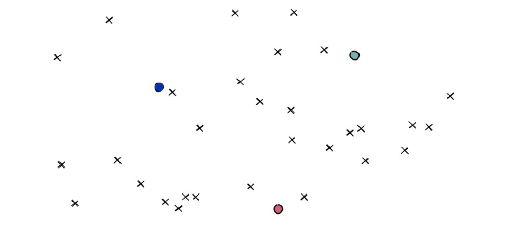
For example, the following set of X marks represents points (or vectors). Suppose we have three centroids:
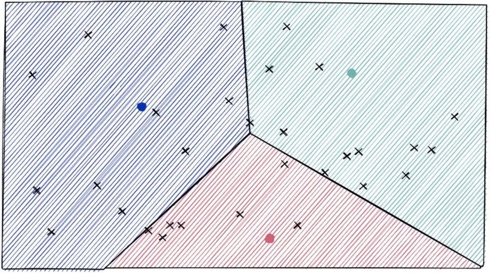
The three centroids partition 3 Voronoi cells, and all points are assigned to their respective Voronoi cells:
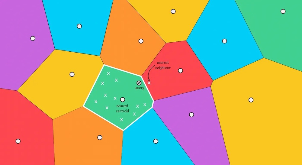
IVFFlat Index Search#
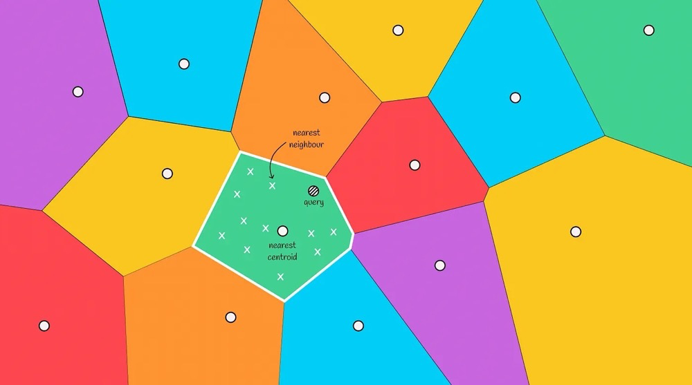
Now there is a query node. Compute its distance to all centroids, find the nearest centroid, and the cell containing that centroid is the region to search next. Finally, within that region, find the neighboring nodes33:
Boundary Problem:
The above search path has a boundary problem. When the query is near a region boundary, if the true nearest node is in another region, the algorithm of “only searching for neighboring nodes within the region” will not find the true nearest neighbor.
The boundary problem is fundamentally because:
The Voronoi diagram only guarantees that the distance from a node to its own region’s centroid is smaller than the distance to other centroids, but it does NOT guarantee that the distance from a node to other nodes in its own region is smaller than the distance to nodes in other regions.
This problem can be mitigated by increasing the number of regions searched. For example, increasing the number of regions searched from 1 to 3:

Increasing the number of search regions is generally set as a parameter in databases, such as ivfflat.probes in pgvector.
IVFFlat Search Summary:
- Compute the distance from the query node to all other centroids, find the nearest one.
- Based on the input parameter for the number of cells to query (e.g., probes), search for neighboring points in the top
probescells.
IVFFlat Index Parameters#
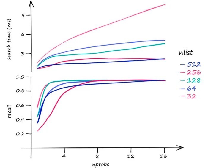
Similarly, vector databases that support IVFFlat indexes generally have at least two parameters: list and probe. These parameters affect index search performance and recall. Here we use Faiss parameters as an example32.
- nlist: Number of regions to construct. Increasing nlist increases the time to search for the nearest centroid but reduces the time to search for nodes within a region.
- nprobe: Number of regions to search. Increasing nprobe increases the number of regions searched, which obviously reduces search performance but improves recall.
Theoretically, for nlist, it’s best to test specifically against the structure of the vector data and the database type — increasing nlist does not always reduce response time. For nprobe, increasing nprobe definitely reduces search performance and improves recall, but making nprobe too large is meaningless and goes against the original intent of ANN.
The following is from Pinecone’s performance testing of the Faiss IVFFlat index:
PQ Product Quantization#
One million dense vectors may require gigabytes of memory, and real-world vectors far exceed this number. Without management, similarity vector search can require enormous amounts of memory — yet RAM is limited. Vector size increases with vector dimensionality and the number of vectors.
Product Quantization (PQ) aims to reduce memory usage and can also improve query speed (because the amount of computation is reduced). PQ is a lossy compression method, which leads to reduced vector retrieval accuracy, but this is acceptable within ANN requirements.
PQ’s algorithm logic is slightly more complex than other algorithms. I strongly recommend this article: Similarity Search, Part 2: Product Quantization34.
PQ Construction#
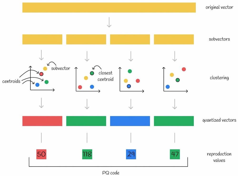
Step description:
- Subvectors — Split the original high-dimensional vector into n low-dimensional sub-vectors.
- Codebook — Use the k-means algorithm (or other algorithms) to compute the Voronoi diagram for each set of all sub-vectors, producing n different Voronoi diagrams. These Voronoi diagrams are the codebooks (assuming each Voronoi diagram has k centroids).
- Clustering — Place the n sub-vectors into their respective already-clustered Voronoi diagrams and compute the nearest centroid.
- Quantized vectors — Take these n nearest centroids as the new vector — the quantized vector.
- Reproduction values — Take the nearest centroid index for each of the n subspaces as new values; the combined new values are called the PQ code.
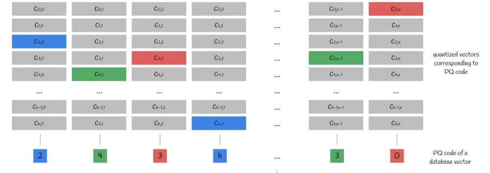
Step 5, reproduction values, in detail:
Based on the n sub-vectors and the k centroids in each subspace, we obtain an n×k centroid matrix. Taking the index of the nearest centroid for each sub-vector gives the PQ code.
(btw: to be rigorous, all element indices in the diagram below should start from 1, not 0.)
The new PQ code is equivalent to a lossy-compressed new vector (reproduction value) of the original vector. New distance calculations can directly compute the L2 distance of the PQ codes.
PQ Retrieval#
Based on the PQ original paper35, there are two PQ retrieval modes:
- Symmetric mode: The distance between vector x and vector y is approximated by the distance between their centroids q(x) and q(y). In other words, the distance between two vectors can be approximated by the distance between their PQ codes.
- Asymmetric mode: The distance between vector x and vector y is approximated by the distance from x to the centroid q(y). In other words, the distance between two vectors can be computed using the original query vector value and the other vector’s PQ code.
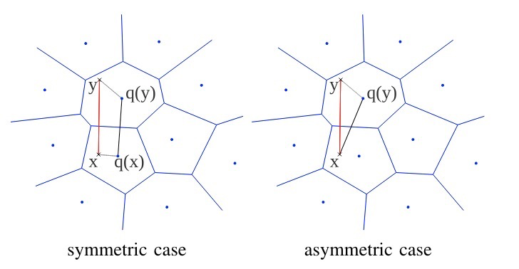
Clearly, the distance accuracy differs between the two modes:
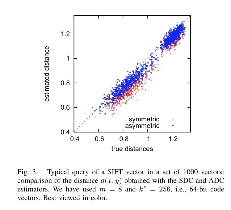
The figure above shows the distance accuracy between two vectors under different modes, with 8 subspaces and 256 centroids. It can be seen that the asymmetric mode has higher accuracy than the symmetric mode.
When comparing distances between two vectors, the symmetric and asymmetric distance computation models are quite useful. However, in the scenario of finding PQ approximate vectors, there are some differences — especially the symmetric mode, where distortion can be quite severe:
The symmetric mode’s query speed is very fast because the code table has already been computed and preserved during the PQ construction process. You only need to first compute the query vector x’s PQ code via the code table (minimal computation), then reverse-lookup the code table to get the corresponding sub-code-table — all vectors in this sub-code-table are approximate vectors at equal distance. This method requires extremely little computation — just a direct table lookup.
The symmetric mode’s distortion is relatively severe (the two figures above don’t fully capture it — imagine it as a Voronoi diagram where one cell contains multiple vectors, and you’ll realize how severe the symmetric distortion can be). The asymmetric mode can slightly alleviate this problem. In asymmetric mode, first compute the PQ code of vector x, then similarly reverse-lookup the code table to get the corresponding sub-code-table, then compute distances between vector x and the vectors in this sub-code-table to obtain KNN. Its computational cost is n×km (n = number of subspaces, km ≈ total vector count / centroid count).
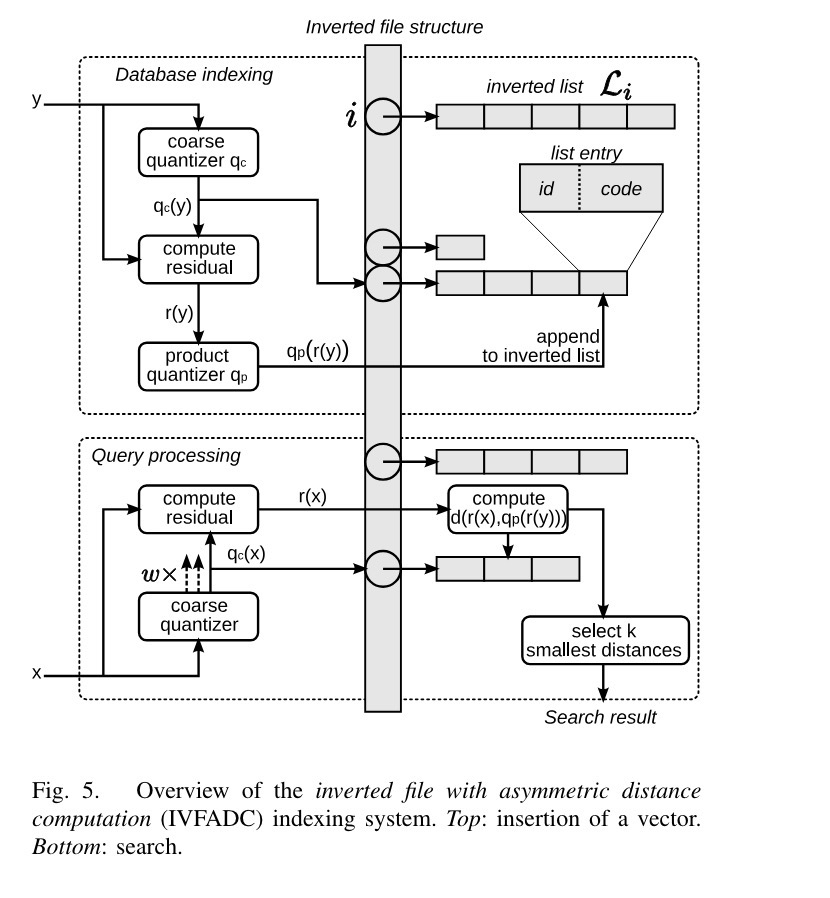
Asymmetric mode requires finding the centroid via the PQ code, then searching for KNN within the subspace where the centroid resides. The distance between the query vector x and an existing vector y is approximated by the distance between x and y’s centroid.
PQ asymmetric retrieval34:
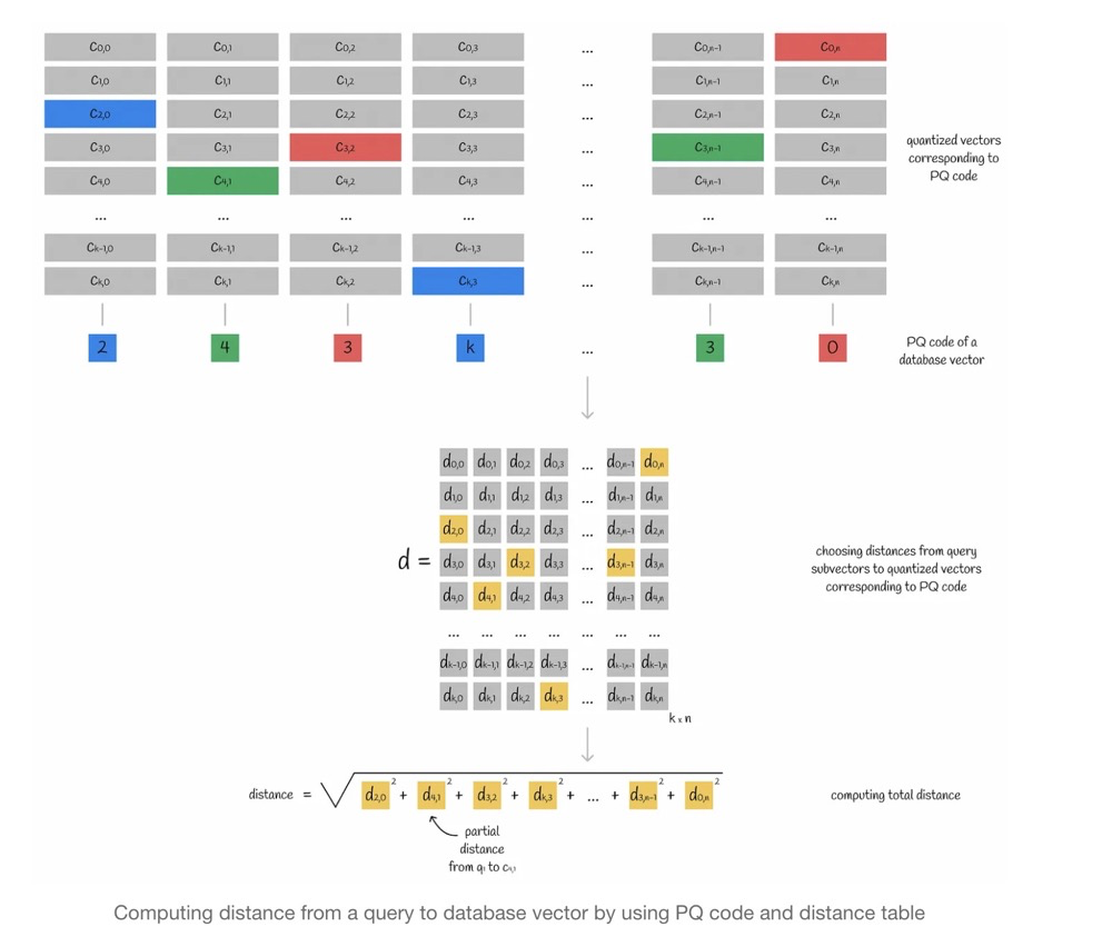
Steps of PQ asymmetric retrieval:
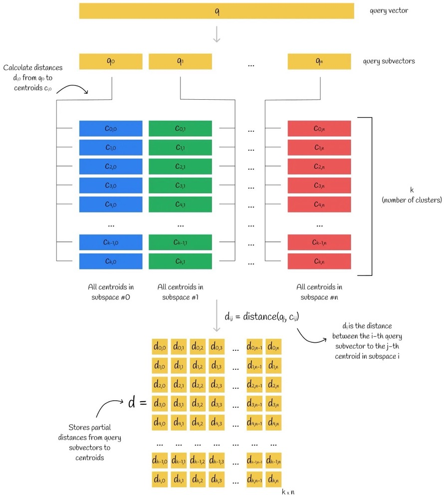
- Split the query vector into multiple sub-vectors.
- Compute the distance between sub-vectors and the centroid matrix.
- Take the nearest centroid in each subspace as the query vector’s PQ code.
- Compute the approximate distance using the query vector and the centroid corresponding to the PQ code. Distances can be computed independently in each subspace and then summed.
As mentioned earlier, asymmetric mode’s approximate distance computation is slightly better than symmetric mode, but in some scenarios, the asymmetric distance can still deviate significantly from the actual distance:
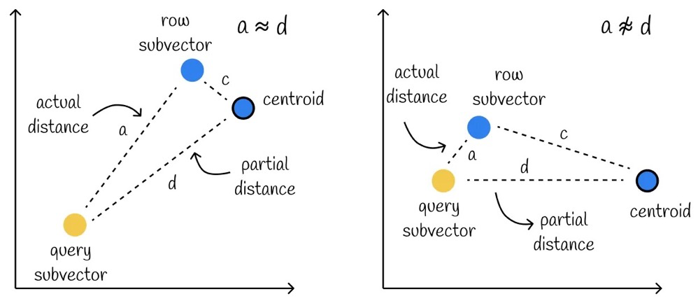
This is easier to understand from the figure above. Within the same cell, the distance between the farthest vector and the centroid can differ significantly from the distance between the closest vector and the centroid. Computing only the partial distance to the centroid cannot capture this difference.
PQ Parameters and Their Impact#
PQ has at least two parameters that significantly affect performance and memory: the number of subspaces m and the number of centroids per subspace k.
Recall:
The product quantizer is parametrized by the number of subvectors m and the number of quantizers per subvector k*, producing a code of length m × log2 k
With m subspaces, each having k* centroids, the length (in bits) of a PQ code is35: $$ code ; length , (bits)=m \cdot \log_2 k^* $$
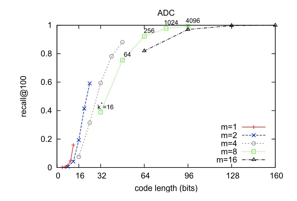
The more subspaces m, the higher the recall; the longer the PQ code, the higher the recall. Longer PQ code essentially means more centroids. Note that the specific values here are based on the paper’s dataset.
Memory and complexity:
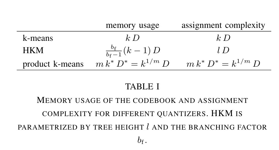
k represents the number of cluster centroids, D represents dimension, m represents the number of subspaces. k* represents centroids within a subspace, D* represents dimensions within a subspace.
For example, with k=2048, D=128, m=8, the complexity is as follows36:
| Operation | Memory and complexity |
|---|---|
| k-means | kD = 2048×128 = 262144 |
| PQ | mkD = (k^(1/m))×D = (2048^(1/8))×128 = 332 |
It can be seen that PQ significantly reduces complexity during search.
DiskANN & Vamana#
The DiskANN original paper Abstract37:
Current state-of-the-art approximate nearest neighbor search (ANNS) algorithms generate indices that must be stored in main memory for fast high-recall search. This makes them expensive and limits the size of the dataset. We present a new graph-based indexing and search system called DiskANN that can index, store, and search a billion point database on a single workstation with just 64GB RAM and an inexpensive solid-state drive (SSD).
At the time (the paper was published in 2019), state-of-the-art ANN algorithms all relied on RAM for high recall and performance. This approach was not only expensive but also limited dataset size. DiskANN requires only 64GB RAM and an affordable SSD.
Vamana Construction#
Vamana iteratively builds a directed graph, starting from a random graph where each node represents a data point in the vector space. Initially, the graph is highly connected — all nodes are connected to each other. The graph is then optimized using an objective function that aims to maximize connectivity between the closest nodes. This is achieved by pruning most random short-range edges while adding certain long-range edges that connect distant nodes (to accelerate graph traversal)37.
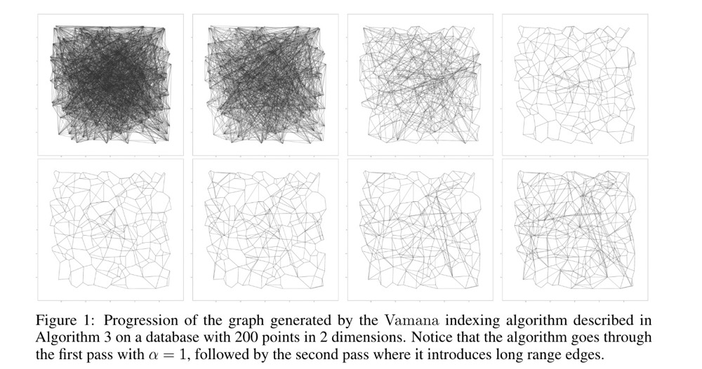
The figure shows 200 2D points after two iterations. The first iteration aggressively prunes edges but also removes long edges that reduce path length; when alpha is increased to relax the pruning condition, long edges are added back38. For the specific algorithm, refer to the paper — this is roughly the idea.
The DiskANN Algorithm#
From the paper’s “The DiskANN Index Design”:
The high-level idea is simple: run Vamana on a dataset P and store the resulting graph on an SSD. At search time, whenever Algorithm 1 requires the out-neighbors of a point p, we simply fetch this information from the SSD. However, note that just storing the vector data for a billion points in 100 dimensions would far exceed the RAM on a workstation! This raises two questions: how do we build a graph over a billion points, and how do we do distance comparisons between the query point and points in our candidate list at search time in Algorithm 1, if we cannot even store the vector data?
Run Vamana on the vector set and store it on SSD. When the dataset is very large, two problems must be addressed:
- How to index such a large-scale dataset with limited memory resources?
k-means + Vamana stacking algorithm: First, use k-means to partition the data into k clusters, then assign each point to the nearest i clusters. Usually, i=2 is sufficient. Build an in-memory Vamana index for each cluster, and finally merge the k Vamana indexes into one.
- If the original data cannot be loaded into memory, how to compute distances during search?
Use compressed vectors (e.g., PQ) and store the compressed vectors in main memory.
If index data is stored on SSD, disk access count and disk read/write requests must be minimized to ensure low search latency; at the same time, lossy compression reduces recall. Therefore, the DiskANN paper proposes three optimization strategies:
- Beam Search: Simply put, preload neighbor information. When searching for point p, if p’s neighbors are not in memory, they must be loaded from disk. Since the time required for a small number of random SSD accesses is roughly the same as the time for a single SSD sector access, the neighbor information of W unvisited points can be loaded in one batch. W should not be set too large or too small. Setting W too large wastes computational resources and SSD bandwidth, while setting it too small increases search latency.
- Caching Frequently Visited Vertices: Aims to reduce disk access count. Cache all points within C hops from the starting point in memory. The value of C is best set between 3 and 4.
- Implicit Re-Ranking Using Full-Precision Vectors: Since PQ is lossy compression, PQ-based distance algorithms only approximate the actual distance. To eliminate this discrepancy, we store the distance from each point to all its neighbors — this is full-precision. As for the implementation principle, in simple terms, it also leverages disk loading efficiency.
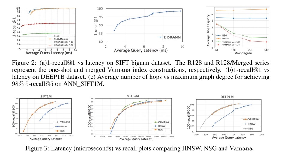
Based on the paper, DiskANN’s execution efficiency and recall outperform IVF and HNSW:
References#
Original article (Chinese): 向量数据库相关概念
Harnessing the Power of LLMs in Practice: A Survey on ChatGPT and Beyond ↩︎
Chih-Hao Liu 66 Classic LLM Papers ↩︎ ↩︎
Jonathan Katz pgconfdev2024 Vectors: How to better support a nasty data type ↩︎
OpenAI recommends using vector databases https://openai.com/index/chatgpt-plugins/ ↩︎
https://en.wikipedia.org/wiki/Vector_(mathematics_and_physics) ↩︎
OpenAI on unit vector usage https://platform.openai.com/docs/guides/embeddings/frequently-asked-questions ↩︎
Pinecone Natural Language Processing for Semantic Search https://www.pinecone.io/learn/series/nlp/dense-vector-embeddings-nlp/ ↩︎
Yao Yuan A Casual Discussion of Various Spaces in Mathematics ↩︎
Jonathan Katz pgconfeu2023 Vectors are the new JSON ↩︎ ↩︎
Vyacheslav Efimov Similarity Search, Part 5: Locality Sensitive Hashing (LSH) ↩︎ ↩︎ ↩︎
Vyacheslav Efimov Similarity Search, Part 6: Random Projections with LSH Forest ↩ ↩︎
earthwjl Delaunay Triangulation Study Notes ↩︎
Vyacheslav Efimov Similarity Search, Part 4: Hierarchical Navigable Small World (HNSW) ↩︎
https://www.pinecone.io/learn/series/faiss/vector-indexes/ ↩︎ ↩︎
Vyacheslav Efimov Similarity Search, Part 1: kNN & Inverted File Index ↩︎
Vyacheslav Efimov Similarity Search, Part 2: Product Quantization ↩︎ ↩︎
Pinecone Faiss Manual https://www.pinecone.io/learn/series/faiss/product-quantization/ ↩︎
DiskANN, A Disk-based ANNS Solution with High Recall and High QPS on Billion-scale Dataset https://milvus.io/blog/2021-09-24-diskann.md ↩︎