Interview questions source: PostgreSQL Apprentice PostgreSQL Interview Questions Collection
Existing answers: Hehuyi_In Learning and Answering PostgreSQL Interview Questions
1. MVCC Implementation and Differences from Oracle#
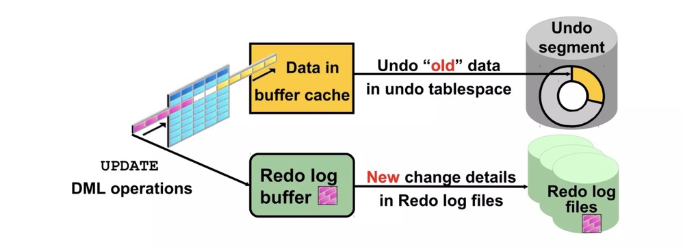
ORACLE and MYSQL both use UNDO to implement multi-version concurrency control. Undo entries are recorded in additional undo tablespaces. If the UNDO segment is insufficient, an ora-01555 error occurs.
 https://www.slideshare.net/AmitBhalla2/less10-undo-15946188
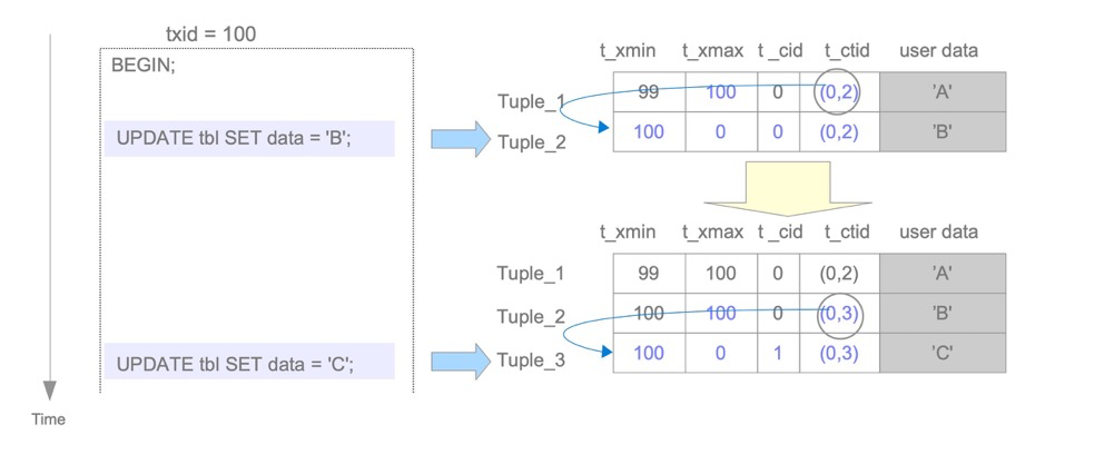
PostgreSQL has no undo mechanism. To ensure transaction rollback, old tuples remain on the table. For example, an update inserts a new row while the old data stays in place. Tuple headers, clog, etc. determine which tuple version is valid. Visibility information in tuple headers includes xmin, xmax, cmin, cmax, infomask, and infomask2, stored in the tuple header.
 https://www.interdb.jp/pg/pgsql05/03.html
Pros/cons: The undo approach requires extra undo space; space management is simpler. However, large transaction rollback is very troublesome since undo segments must be rolled back. The new-tuple approach makes large transaction rollback very fast, but this method creates dead tuples, requiring a vacuum mechanism to clean them. Vacuum freeze itself isn’t directly related to dead tuple cleanup (though both are vacuum processes); freeze prevents transaction ID wraparound.
2. Why Table Bloat Occurs and Its Hazards#
Why table bloat?
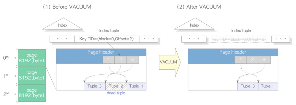
As above, due to PostgreSQL’s unique MVCC mechanism, delete doesn’t truly remove tuples, and update equals delete+insert. Old tuples cannot be removed by DML statements, so space only “grows” without “cleaning” — this is table bloat. Vacuum is generally needed to clean dead tuples and mark space as available; or vacuum full rewrites the table for compaction.
Hazards of table bloat:
- Excessive table space usage
- SQL performance degradation
- Large tables cause longer vacuum cleanup times; vacuum full blocking time also increases, though pg_repack can replace vacuum full to reduce blocking
Handling table bloat:
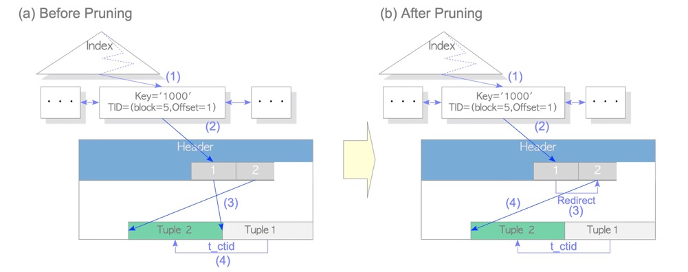
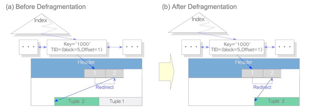
- Manual vacuum
- Does not block queries or DML operations
- Does not immediately reclaim space, only marks it as available
- If the last page of a table has no tuples, that page gets truncated
 (https://www.interdb.jp/pg/pgsql06.html)
- Autovacuum
- Autovacuum automatically invokes vacuum for concurrent cleanup as needed
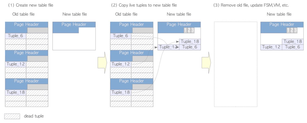
- Manual vacuum full
- 8-level lock, blocks everything
- Table is completely rewritten; corresponding OS files are cleaned and rebuilt
- Rebuilds indexes, FSM (free space map), VM (visibility map)
- pg_repack and other manual table rebuilds
- pg_repack only has a brief lock during the final table switch
- Other tools with data sync and switch capabilities
Avoiding table bloat:
Generally, autovacuum handles table bloat, but cleanup may not proceed smoothly in some scenarios:
- Autovacuum worker isn’t running
- Both
autovacuumandtrack_countsmust be enabled for autovacuum to work autovacuum_max_workersmust be set high enough; multiple workers may be needed simultaneously- Table hasn’t reached vacuum threshold — rows deleted/updated: threshold =
autovacuum_vacuum_threshold+autovacuum_vacuum_scale_factor* tuples autovacuum_vacuum_insert_thresholdandautovacuum_vacuum_insert_scale_factorrepresent insert thresholds (same algorithm). Insert-triggered vacuum thresholds theoretically have little to do with bloat cleanup since inserts don’t generate dead tuples. However, to prevent wraparound issues from not being handled in time, pg13 added this parameter (reference: postgresql-autovacuum-insert-only-tables)autovacuum_naptimeis the autovacuum launcher cycle. If set too large,autovacuum_max_workersmay be sufficient and tables may meet thresholds, but the launcher hasn’t woken workersvacuum_defer_cleanup_agedelays vacuum cleanup by N transactions (originally designed to alleviate standby query conflicts; sincehot_standby_feedbackand replication slots exist, pg16 removed this parameter)
- Disable or adjust cost-based vacuuming to make autovacuum faster
- Cost-based vacuuming may be enabled to reduce vacuum’s IO impact. When vacuum/autovacuum reaches the cost limit, it sleeps for
autovacuum_vacuum_cost_delay(orvacuum_cost_delay) milliseconds.vacuum_cost_delaydefaults to 0 (disabling cost-based vacuuming);autovacuum_vacuum_cost_delayat -1 means using thevacuum_cost_delaysetting. Disable delay or reduce the delay value - If cost-based vacuuming is enabled, reasonably increase
vacuum_cost_limittrigger threshold and reduce thevacuum_cost_page_dirty,vacuum_cost_page_miss,vacuum_cost_page_hitvalues that count toward the limit
- Active transactions preventing vacuum
- Business long transactions not finished. Application-side transactions shouldn’t run too long; database-side can kill sessions: 1) manual kill 2) set
idle_in_transaction_session_timeoutto limit idle time 3) setold_snapshot_thresholdto limit SQL execution (not recommended before PG14) - Unclosed cursors
hot_standby_feedbackenabled: primary records catalog_xmin, standby long queries prevent primary cleanup- Remove unused replication slots
- Orphan transactions. Prepared transactions are explicit 2PC transactions inside PG. If a prepared transaction is opened but not completed, and prepared transactions are unrelated to sessions, orphan transactions block indefinitely
- pg_dump logical backup opens implicit repeatable read isolation level; transaction not finished
- Performance aspects
maintenance_work_memis memory for maintenance operations like vacuum; default 64MB can be increased. Or useautovacuum_work_memseparately for autovacuum workers; default -1 means usingmaintenance_work_mem- Large table vacuum is especially slow; since vacuum can’t parallelize on the same table, convert large tables to partitioned tables so vacuum can run in parallel across partitions
- Good IO system
- Adjust per-table autovacuum parameters
- Global autovacuum settings may not suit certain business tables; adjust per-table autovacuum parameters to increase vacuum trigger probability
- Manual vacuum
- Autovacuum is generally unpredictable; for special business tables, manual vacuum
- Run manual vacuum during low-traffic periods, optionally with freeze and analyze
The above handles 99.99% of table bloat problems. One type of bloat is harder to address: with cost-based vacuuming disabled, autovacuum dead tuple cleanup speed cannot keep up with generation speed. Essentially, too many concurrent update (or insert+delete) transactions mean this round of vacuum hasn’t finished cleaning available space before massive updates generate new space and dead tuples, causing continuous bloat. Solutions:
- Convert to partitioned tables for vacuum parallelism (only meaningful if updates are distributed across partitions)
- Run vacuum full or pg_repack during off-peak hours to thoroughly clean table holes
- 24/7 high-concurrency tables are unlikely; if they exist, restructure to multi-table writes or move to caching systems like Redis
Unveiling the Mystery of Table Bloat
https://www.interdb.jp/pg/pgsql06.html
https://www.postgresql.org/docs/16/routine-vacuuming.html
https://www.postgresql.org/docs/16/runtime-config-autovacuum.html
https://www.postgresql.org/docs/16/runtime-config-resource.html#GUC-VACUUM-COST-DELAY
3. Long Transaction Hazards and How to Trace Them#
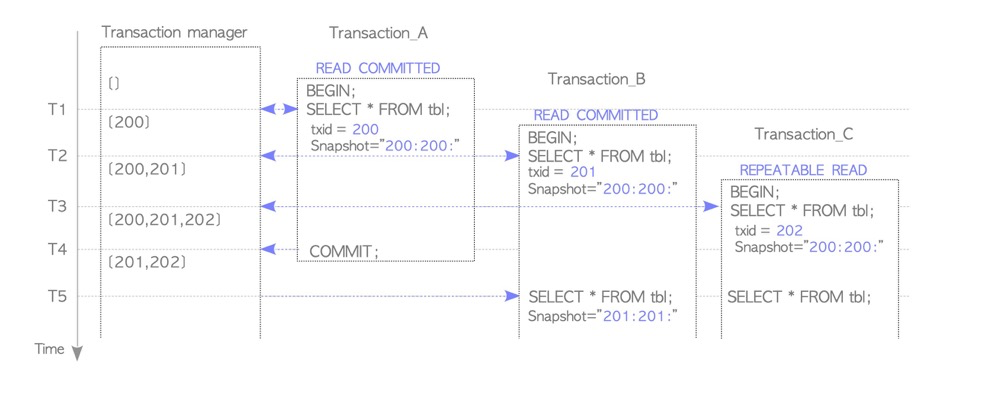
Regular queries don’t generate transaction IDs but virtual transaction IDs (vxid). Virtual transaction IDs consist of backendID and a backend-local counter, unrelated to transaction ID (XID). However, although queries don’t generate transaction IDs, they hold snapshots for visibility checks. Snapshots contain tuple xmin and other information.
(https://www.interdb.jp/pg/pgsql05/05.html)
So long transaction issues involve both DML and query statements, though their lock types differ.
Long transaction hazards:
- Blocks vacuum cleanup, causing table bloat, excessive space usage, and SQL performance degradation
- Blocks other lock requests; e.g., DDL must check for long transactions before execution, otherwise long waits for higher-level locks cause lock escalation
- Long transactions cause create index concurrently to fail, leaving invalid indexes
- Occupies connection pool (though mainly a long-connection issue)
- Logical decoding data spilling to disk causing replication lag, also related to large transactions
- A long transaction with a savepoint subtransaction can cause query performance cliffs (reference: Why we spent the last month eliminating PostgreSQL subtransactions)
How to trace long transactions:
- pg_stat_activity: check xact_start for transaction start time, state_change for whether transaction is still running
4. Subtransaction Hazards and Considerations#
Subtransaction hazards:
- Excessive transaction ID consumption, premature wraparound handling. Each subtransaction consumes one XID
- PGPROC_MAX_CACHED_SUBXIDS overflow causing performance degradation. Each backend has a subtransaction cache of
PGPROC_MAX_CACHED_SUBXIDS, fixed at 64 subtransactions (hardcoded). Exceeding 64 subtransactions spills to thepg_subtransdirectory (reference: PostgreSQL Subtransactions Considered Harmful) - Using subtransactions with FOR UPDATE explicit row locks causes dramatic database performance degradation (reference: Notes on some PostgreSQL implementation details)
- A long transaction with a savepoint subtransaction can also cause query performance cliffs (reference: Why we spent the last month eliminating PostgreSQL subtransactions)
Usage recommendations:
- Subtransaction usage is discouraged given the above hazards
- If standby query workloads exist, prohibit subtransactions
- If subtransactions are still needed, keep them under 64 (preferably much lower)
- Besides explicit savepoints, subtransactions can also arise from exceptions, frameworks, and tools
5. Which Schema Changes Are Non-Online#
All schema changes are non-online because all ALTER TABLE operations require an 8-level lock. However, some schema changes themselves take a long time or cause slow queries afterward. So this question can be reframed as three sub-questions:
Impact on indexes? Impact on statistics? Does it require rewriting the table, causing long-held 8-level locks?
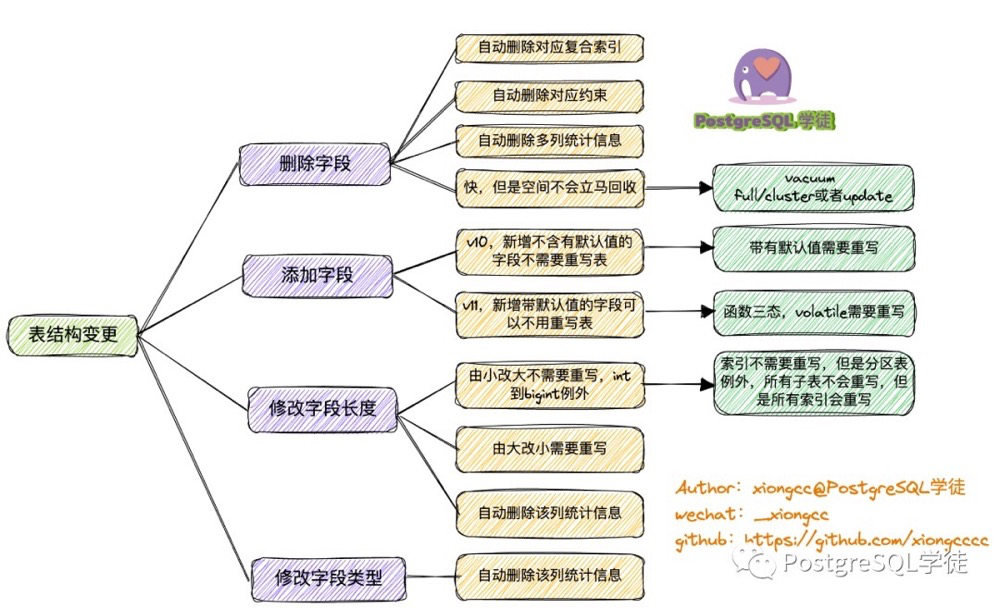
Summary:
- Dropping a column completes immediately, but watch for composite index and multi-column statistics invalidation to avoid SQL performance avalanches
- Adding a column with a default value: 1) Pre-pg10 requires table rewrite 2) pg11+: only volatile function defaults require table rewrite. Also, statistics won’t be immediately available for the new column
- Changing column length: enlarging (except int to bigint) doesn’t rewrite the table; shrinking requires table rewrite; column statistics invalidated
- Changing column type: table rewrite; statistics invalidated
- Adding constraints to existing columns scans the table, watch for scan duration (e.g.,
ADD CONSTRAINT,SET NOT NULL) - Adding defaults to existing columns completes immediately (e.g.,
SET/DROP DEFAULT) - SET { LOGGED | UNLOGGED } rewrites the table
- Storage parameter changes depend on what’s changing. E.g., fillfactor and autovacuum parameters are online, non-8-level-lock, immediate (reference: Storage Parameters)
6. Physical Backup Considerations (pg_start_backup)#
(https://postgrespro.com/media/2022/03/24/pgpro-backup-methods%20(1).pdf)
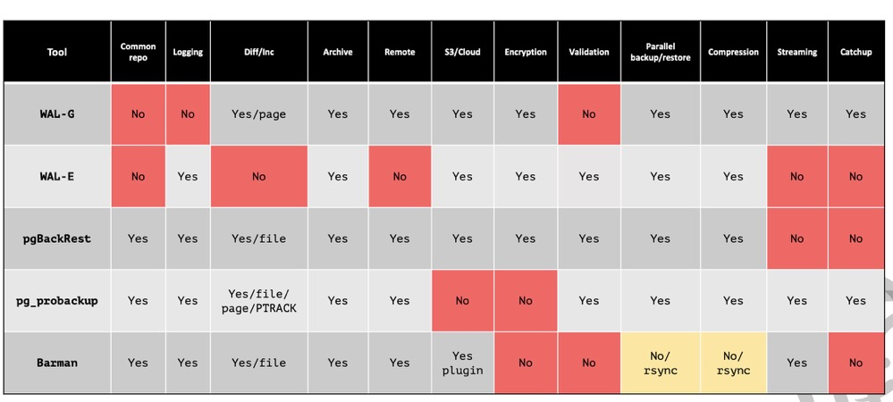
PG physical backup:
- Block-level backup, generally doesn’t support per-database backup (except pg_probackup)
- Exclusive mode is unnecessary because: 1) only works on primary 2) doesn’t allow parallel backup 3) created backup label may prevent primary instance recovery 4) functionally identical to non-exclusive backup. PG9.6 added non-exclusive mode; PG15 removed exclusive mode
- If explicitly using pg_start_backup(), must explicitly use pg_stop_backup() to end backup mode (function names differ slightly in PG15+)
- FPI (full page image) is force-enabled during backup, even if full_page_writes is off
- All tools (maybe) call pg_stop_backup() before backup starts for a checkpoint to flush dirty data, and back up all WAL from start to end, even newly generated WAL during backup, ensuring data consistency and PITR
pg_basebackup:
- Native, built-in
- Wraps pg_start_backup and pg_stop_backup commands
- PG17+ supports incremental backup and backup set merging
- Consumes one walsender process
pg_probackup:
- Very powerful: supports incremental backup, incremental restore, parallelism, backup set merging, backup verification, remote backup, per-database restore, etc.
- BUG: address space cannot exceed 4GB, fixable by modifying source code
pgBackRest:
- Also very powerful
- Prerequisite: SSH must be configured from backup server to database host
https://developer.aliyun.com/article/59359
https://www.postgresql.org/docs/current/app-pgbasebackup.html
https://www.enterprisedb.com/blog/exclusive-backup-mode-finally-removed-postgres-15
https://github.com/MasaoFujii/pg_exclusive_backup
https://github.com/postgrespro/pg_probackup
https://pgbackrest.org/user-guide.html
7. How Logical Backup Ensures Consistency#
- pg_dump completes a full backup within a single transaction, with isolation level serializable or repeatable read
- Before backing up data, pg_dump acquires ACCESS SHARE locks on target objects to prevent table drops
Additional logical backup considerations:
- Watch for lock conflicts during export
- If DDL operations are needed, avoid full-database or long-duration backups; split the backup into multiple tasks, e.g., one table per pg_dump invocation
https://developer.aliyun.com/article/14582
8. Causes of WAL Accumulation#
- Invalid replication slots
- Logical replication with long transactions
- Excessively large wal_keep_size
- Excessively small archive_timeout, forcing WAL switches and archiving (equivalent to pg_switch_xlog() + archiving)
- Archive failures generating .ready files
- Single-process archiving can’t keep up
- FPI full page writes (check for overly frequent checkpoints, UUID-like scattered write patterns)
9. Hazards of Long Connections#
- When PG acquires snapshot data, it must scan all backend process transaction states. Too many connections degrade performance (recommended max ~1000; pg14 optimized but still not recommended to exceed)
- relcache/syscache doesn’t release cached metadata, and each process caches independently, causing high memory consumption
10. Role of Infomask Flags#
- Infomask provides transaction, lock, and tuple status information, such as whether a transaction is committed/aborted, row lock info, HOT info, column count, etc.
- The header has two infomasks:
infomaskandinfomask2. They store different information, with different bits representing different meanings - Hint bits also write transaction info to infomask, so visibility can be determined from tuple headers alone without accessing clog
11. How NULL Values Are Stored and Whether Indexes Store NULLs#
How NULL values are stored:
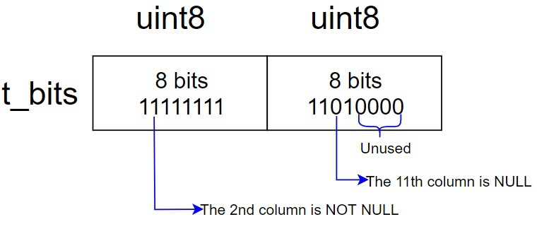
- NULL is stored in the tuple header, not the tuple data area
- One bit in infomask marks whether the tuple contains NULLs
- t_bits has n*8 bits (n integer; e.g., a 10-column table has 16-bit t_bits), with a bitmap representing which columns are NULL
Whether indexes store NULL values:
- PostgreSQL indexes store NULL values; Oracle indexes don’t
- Storage position depends on (NULLS FIRST or NULLS LAST)
https://www.highgo.ca/2020/10/20/the-way-to-store-null-value-in-pg-record/
12. Why Full Page Writes Are Needed#
The official documentation’s introduction to full page writes is fairly general:
This is needed because a page write that is in process during an operating system crash might be only partially completed, leading to an on-disk page that contains a mix of old and new data. The row-level change data normally stored in WAL will not be enough to completely restore such a page during post-crash recovery. Storing the full page image guarantees that the page can be correctly restored, but at the price of increasing the amount of data that must be written to WAL. (Because WAL replay always starts from a checkpoint, it is sufficient to do this during the first change of each page after a checkpoint)
OS file pages are typically 4KB, while PG pages are typically 8KB. Partial writes can occur, where a disk data page contains both old and new data, causing data loss during recovery. Hence the need for full page writes.
Partial writes are closely related to disk characteristics. Detailed answers are difficult; reference roger’s article. Summary:
- Partial writes relate to whether the disk supports atomic writes
- Partial writes relate to whether OS block size matches database block size. Oracle/PG blocks default to 8KB, MySQL to 16KB, OS to 4KB. A database’s minimum IO requires multiple OS calls
- For PG, if a data page experiences partial write, it can recover using full page images in WAL
- For MySQL, there’s a double write mechanism. The double write buffer is on-disk space, written sequentially before data pages to mitigate partial write
- For Oracle, much work has been done but no obvious solution exists. However, Oracle supports block-level recovery to replace corrupted data blocks
Different DBs adopt different approaches to reduce partial writes. PG writes the entire data page to WAL logs, but this causes WAL write amplification. This can be mitigated through various means.
How to perfectly solve the partial write problem?
- Atomic write-capable devices
- OS minimum IO matching database minimum IO
http://www.killdb.com/2020/04/05/double_write_partial_write_oracle_mysql_postgresql/
13. Various Causes of Index Invalidation#
Index invalidation:
- CREATE INDEX CONCURRENTLY can leave an invalid index due to deadlock or unique index check failure; invalid indexes still get updated
- Invalid indexes on partitioned parent tables indicate some partitions have the index while others don’t
Index not being used:
- Inaccurate statistics
- Selectivity
- Data skew
- Soft parsing: first 5 times cached different execution plans
- Leftmost prefix principle
- Insufficient data (hash or full scan not slower than index)
- Functions (unless a matching immutable function index exists), implicit conversions, operations, LIKE with leading ‘%’…
- Data type mismatch
- Collation mismatch (less of an issue in PG since database collation can’t change after creation; data within one database shares the same collation; cross-database access is normally impossible)
- SQL collation sort differing from index collation sort
- LIKE only usable with collation C or pattern index
- High correlation: index logical order vs data physical order correlation; accessing scattered data via index
- LIMIT xx ORDER BY column1, MIN/MAX needing TOP N scenarios where the optimizer chooses another index
14. Role of Commit Log#
Commit log records transaction status. During the next visibility check on a table, hint bits are triggered, writing clog transaction status to the tuple header.
Why not write transaction status to the tuple header immediately? Hint bits immediate update performs very poorly, so transaction status is first placed in clog, reducing PGXACT contention and improving performance.
15. Database Join Methods and Their Applicable Scenarios#
1.1 Nested Loop Join
lzldb=# explain select a from lzl1,t3 where lzl1.col1=t3.a::text;
QUERY PLAN
-----------------------------------------------------------
Nested Loop (cost=0.00..2.29 rows=10 width=4)
Join Filter: ((lzl1.col1)::text = (t3.a)::text)
-> Seq Scan on t3 (cost=0.00..1.01 rows=1 width=4)
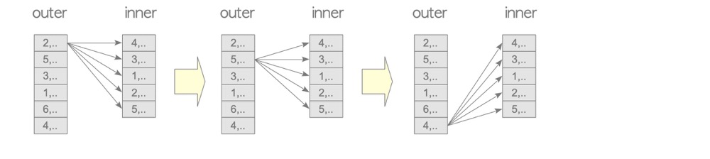
-> Seq Scan on lzl1 (cost=0.00..1.10 rows=10 width=2)The driving table (outer in the diagram, first table in the plan) matches each row against every row of the driven table (inner, second table in the plan). The driving table is scanned once; the driven table is scanned N times (N = driving table rows).
NL suits almost all scenarios; it’s the simplest brute-force join. Generally smaller tables serve as the driving table (actually neither table should be too large, unless other join types don’t apply).
1.2 Materialized Nested Loop Join
testdb=# EXPLAIN SELECT * FROM tbl_a AS a, tbl_b AS b WHERE a.id = b.id;
QUERY PLAN
-----------------------------------------------------------------------
Nested Loop (cost=0.00..750230.50 rows=5000 width=16)
Join Filter: (a.id = b.id)
-> Seq Scan on tbl_a a (cost=0.00..145.00 rows=10000 width=8)
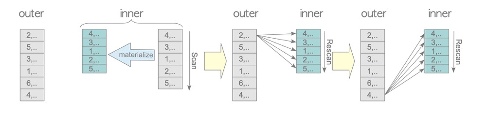
-> Materialize (cost=0.00..98.00 rows=5000 width=8)
-> Seq Scan on tbl_b b (cost=0.00..73.00 rows=5000 width=8)If the driven table (inner) needs multiple scans, physical IO each time would be very slow (and seems silly). Materialize scans the driven table into memory (work_mem), performing only one physical table scan, allowing the driven table to be accessed multiple times in memory.
This scenario is very common in real-world workloads.
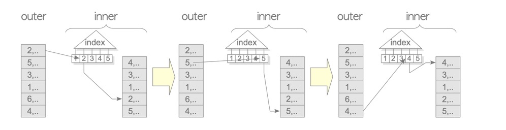
1.3 Indexed Nested Loop Join (inner indexed)
testdb=# EXPLAIN SELECT * FROM tbl_c AS c, tbl_b AS b WHERE c.id = b.id;
                                   QUERY PLAN
--------------------------------------------------------------------------------
 Nested Loop  (cost=0.29..1935.50 rows=5000 width=16)
   ->  Seq Scan on tbl_b b (cost=0.00..73.00 rows=5000 width=8)
   ->  Index Scan using tbl_c_pkey on tbl_c c  (cost=0.29..0.36 rows=1 width=8)
         Index Cond: (id = b.id)
1.4 NL Variants
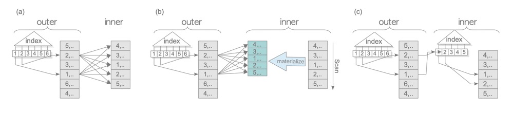
All are essentially NL; the main variations are whether indexes are used on either table and whether Materialize is applied.
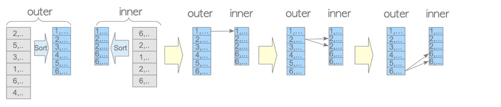
2.1 Merge Join
testdb=# EXPLAIN SELECT * FROM tbl_a AS a, tbl_b AS b WHERE a.id = b.id AND b.id < 1000;
                               QUERY PLAN
-------------------------------------------------------------------------
 Merge Join  (cost=944.71..984.71 rows=1000 width=16)
   Merge Cond: (a.id = b.id)
   ->  Sort  (cost=809.39..834.39 rows=10000 width=8)
         Sort Key: a.id
         ->  Seq Scan on tbl_a a  (cost=0.00..145.00 rows=10000 width=8)
   ->  Sort  (cost=135.33..137.83 rows=1000 width=8)
         Sort Key: b.id
         ->  Seq Scan on tbl_b b  (cost=0.00..85.50 rows=1000 width=8)
               Filter: (id < 1000)
(9 rows)
In merge join, both the driving and driven tables must be sorted first (both tables have Sort in the plan) before matching. Advantage: fewer table scans and matches than NL. Disadvantage: sorting required.
Since indexes are sorted, and SQL may include DISTINCT, GROUP BY, SORT, MAX/MIN etc. requiring ordering, merge join is also common.
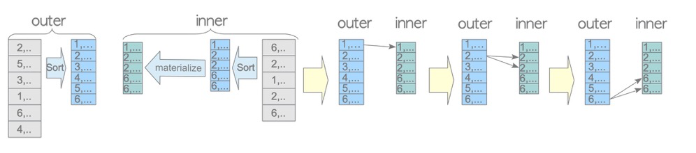
2.2 Materialized Merge Join
testdb=# EXPLAIN SELECT * FROM tbl_a AS a, tbl_b AS b WHERE a.id = b.id;
                                    QUERY PLAN
-----------------------------------------------------------------------------------
 Merge Join  (cost=10466.08..10578.58 rows=5000 width=2064)
   Merge Cond: (a.id = b.id)
   ->  Sort  (cost=6708.39..6733.39 rows=10000 width=1032)
         Sort Key: a.id
         ->  Seq Scan on tbl_a a  (cost=0.00..1529.00 rows=10000 width=1032)
   ->  Materialize  (cost=3757.69..3782.69 rows=5000 width=1032)
         ->  Sort  (cost=3757.69..3770.19 rows=5000 width=1032)
               Sort Key: b.id
               ->  Seq Scan on tbl_b b  (cost=0.00..1193.00 rows=5000 width=1032)
(9 rows)
Materialize doesn’t reduce table scans (both tables scanned once), but the sort operation can happen in the backend’s work_mem for better efficiency; if exceeding work_mem, disk sort is used.
2.3 Merge Join Variants
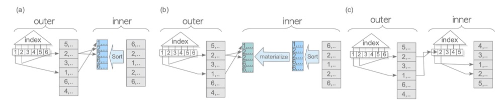
Similar to NL variants, mainly Materialize and index usage. When using indexes, since the index is inherently ordered, no extra sorting is needed:
                                      QUERY PLAN
--------------------------------------------------------------------------------------
 Merge Join  (cost=135.61..322.11 rows=1000 width=16)
   Merge Cond: (c.id = b.id)
   ->  Index Scan using tbl_c_pkey on tbl_c c  (cost=0.29..318.29 rows=10000 width=8)
   ->  Sort  (cost=135.33..137.83 rows=1000 width=8)
         Sort Key: b.id
         ->  Seq Scan on tbl_b b  (cost=0.00..85.50 rows=1000 width=8)
               Filter: (id < 1000)
(7 rows)
So indexes and Materialize are very common in merge joins.
3.1 Hash Join
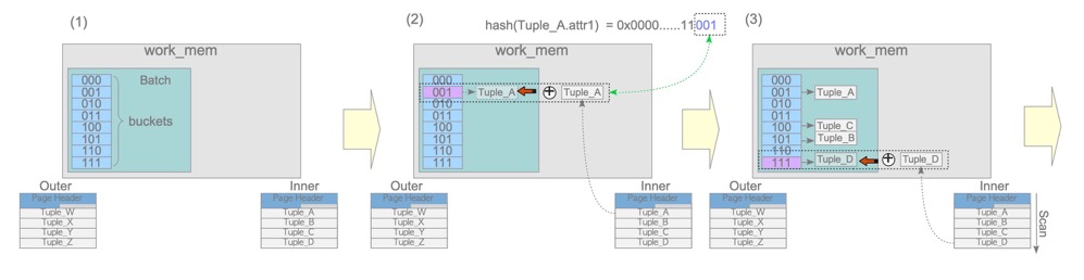
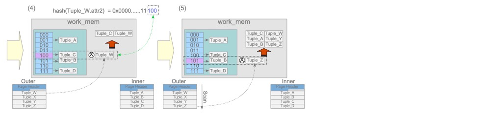
Hash join consists of build and probe phases.
The build phase places the driving table (inner in the diagram, second row in the plan!) into work_mem; the probe phase compares hash values.
- Hash join only possible with ‘=’ conditions
- Hash join consumes memory; generally both tables aren’t very large
- Note: the driving table (hash build table) is the second row in the plan, opposite of NL
3.2 Hybrid Hash Join with Skew
Not fully understood; appears to support spilling to disk. To be revisited.
https://www.interdb.jp/pg/pgsql03/05/01.html
16. Applicable Scenarios for Various Index Types (HASH/GIN/BTREE/GIST/BLOOM/BRIN)#
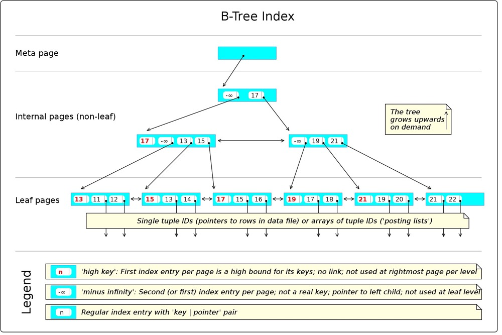
(1) BTREE
https://en.wikibooks.org/wiki/PostgreSQL/Index_Btree
Possible usage patterns:
< <= = >= > IS NULL IS NOT NULL LIKE 'foo%'- A meta node points to the root node
- Leaf node access complexity O(logN), N being row count
- Inherently sorted, easily used by ORDER BY, MIN/MAX, GROUP BY, merge joins, etc.
- Default index type, most common. Structure is similar across databases with leaf node structure differences (MySQL secondary index leaf nodes store index key + primary key, then access clustered index via primary key; Oracle index leaf nodes store index key + rowid; PG index leaf nodes store index key + tid)
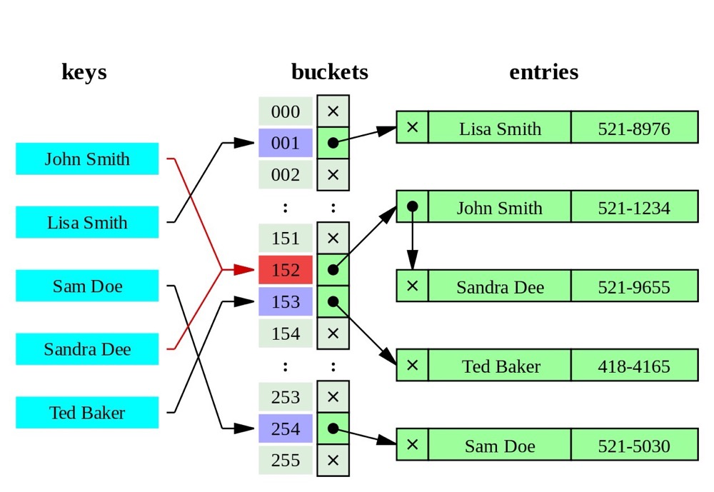
(2) HASH
(https://leopard.in.ua/2015/04/13/postgresql-indexes)
Index data is converted to 32-bit hash values stored in corresponding hash buckets; different hash values point to their respective data rows.
- Complexity O(1)
- Hash indexes can only be used for
=conditions - When key values are large, they’re generally smaller than BTREE indexes and don’t need character-by-character comparison like BTREE, offering better efficiency. So hash indexes suit scenarios with large key values
(3) GIST
GIST (Generalized Search Tree) is similar to BTREE, also a balanced tree. GIST isn’t actually one index type but a framework containing many index strategies: R-TREE, RD-TREE. Unlike BTREE using =, > etc. for numeric/character data, GIST excels at geographic, text, image, and similar data. Geographic operators include: <-> distance calculation, << left-of check, @> contains check, etc.
GIST excels at:
- GIS data processing (similar data processing also possible, e.g., digoal-GIST index for IP range query optimization)
- Nearest-neighbor algorithms (pg_vector and similar vector data; to be researched)
- Full-text search (seems to need contrib/intarray)
RTREE:
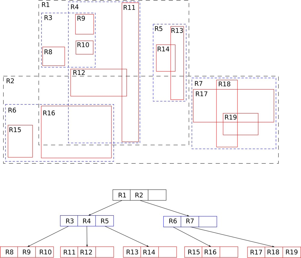
(https://en.wikipedia.org/wiki/R-tree)
The most common index for GIS data is RTREE. Two-dimensional spatial data consists of coordinates; scanning coordinates one by one to find locations is slow. BTREE isn’t suitable for such data, so RTREE emerged. RTREE’s core concept is grouping nearby points using rectangles at different hierarchy levels; finer grouping yields more precise positioning.
https://postgrespro.com/blog/pgsql/4175817
(4) SP-GIST:
Space-Partitioned GIST is similar to GIST, also an index creation framework. SP-GIST suits structures that partition space into non-overlapping regions (unlike RTREE which overlaps), such as quadtrees, k-d trees, and radix trees.
Quadtrees:
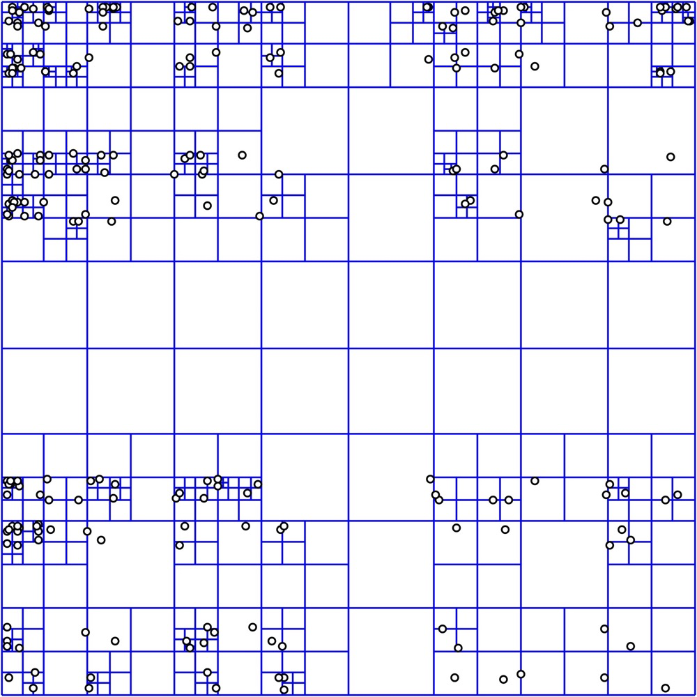
(https://en.wikipedia.org/wiki/Quadtree)
Q-TREE comes in square, rectangular, and various shapes. The most “orthodox” Q-TREE as shown above generally has these properties:
- Each internal node has four children
- Index follows depth structure to locate data
K-d trees:
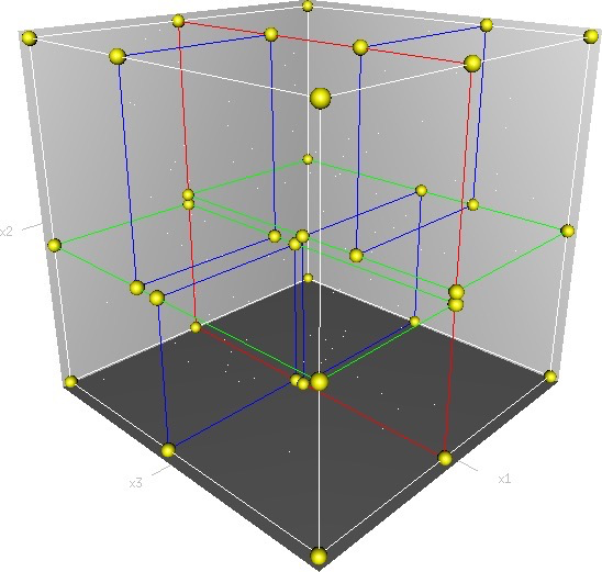
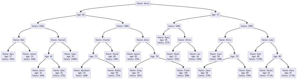
(https://en.wikipedia.org/wiki/K-d_tree)
K-dimensional trees manage multi-dimensional points using multi-dimensional space concepts; each non-leaf node is split in two. For example, the 3D space diagram above is a 3-dimensional k-d tree model: first split (red) divides the entire space in half; second split (green) divides subspaces in half… until no further division is possible. The second diagram shows the tree structure of a 3D k-d tree (don’t mistake it for BTREE!); this tree has only 3 dimensions: Name, Age, Salary.
Radix-tree:
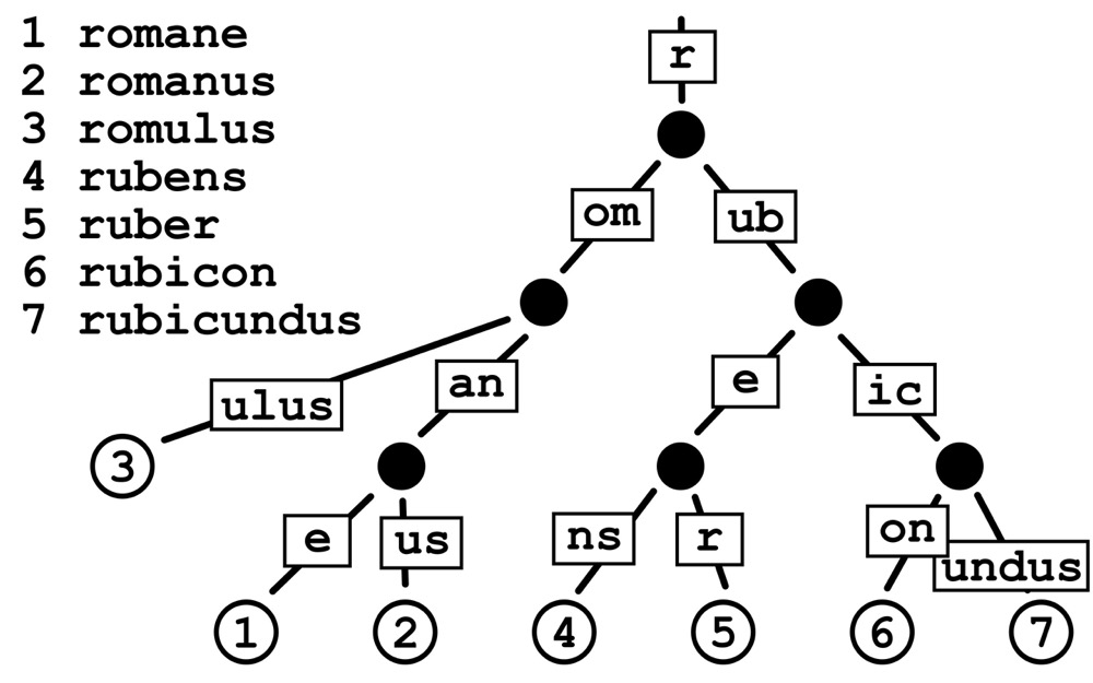
(https://en.wikipedia.org/wiki/Radix_tree)
Radix: each child synthesizes its parent. Key lookup complexity is O(path length); if common prefixes exist, complexity is higher.
https://postgrespro.com/blog/pgsql/4220639
(5) GIN
BTREE and GIST have very low query efficiency when there are very many key-value entries. GIN (Generalized Inverted Index) excels at such scenarios: array, full text, and JSON retrieval operations. Both GIST and GIN are generalized/framework-based, supporting multiple data index types; both also support full-text indexing. GIN only supports Bitmap scans.
PostgreSQL natively supports many operators, some of which are GIN-related data type operators:
- Array operators, e.g.,
@>whether array1 contains array2;unnestexpand array - Full-text search operators, e.g.,
@@whether tsvector matches tsquery - Also some JSON operators
PG supports two data types for full-text search: tsvector and tsquery
1. tsvector:
tsvector tokenizes text with deduplication and sorting, using tsvector_ops operators. Example tokenization:
SELECT 'The Fat Rat is a Rat'::tsvector;
          tsvector
----------------------------
 'Fat' 'Rat' 'The' 'a' 'is'
::tsvector tokenization is generally not the final form; to_tsvector normalizes tokens (final form), showing token positions:
SELECT to_tsvector('english', 'The Fat Rat is a Rat');
    to_tsvector
-------------------
 'fat':2 'rat':3,6
Note ’the’, ‘is’, ‘a’, and case are all removed — this is to_tsvector’s rule, matching real-world scenarios since full-text search typically targets words.
2. tsquery:
Normally you can search tokenized text by word:
SELECT to_tsvector('The Fat Rat is a Rat') @@ 'rat';
 ?column?
----------
 t
To search for “contains both fat and rat”, simple word input won’t work — tsquery operates on the tokens being searched.
tsquery can be composed with & (AND), | (OR), ! (NOT), <-> (FOLLOWED BY). Examples:
SELECT to_tsvector('The Fat Rat is a Rat') @@ to_tsquery( 'fat&rat' );
 ?column?
----------
 t
SELECT to_tsvector('The Fat Rat is a Rat') @@ to_tsquery( 'fat&rat&cat');
 ?column?
----------
 f
 SELECT to_tsvector('The Fat Rat is a Rat') @@ to_tsquery( 'rat<->fat');
 ?column?
----------
 f
Fulltext GIN:
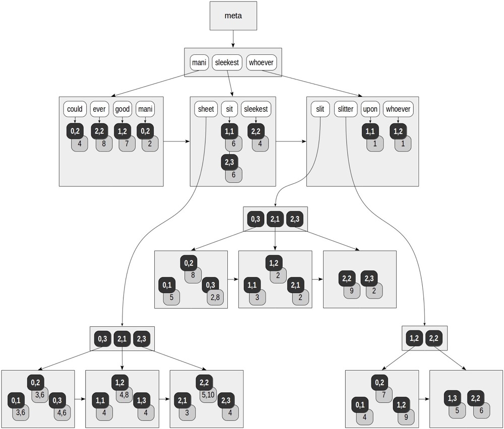
Full-text GIN indexes first tokenize the indexed field (to_tsvector). Example: doc_tsv below is the tokenized state of left:
  ctid |         left         |                         doc_tsv
-------+----------------------+---------------------------------------------------------
 (0,1) | Can a sheet slitter  | 'sheet':3,6 'slit':5 'slitter':4
 (0,2) | How many sheets coul | 'could':4 'mani':2 'sheet':3,6 'slit':8 'slitter':7
 (0,3) | I slit a sheet, a sh | 'sheet':4,6 'slit':2,8
 (1,1) | Upon a slitted sheet | 'sheet':4 'sit':6 'slit':3 'upon':1
 (1,2) | Whoever slit the she | 'good':7 'sheet':4,8 'slit':2 'slitter':9 'whoever':1
 (1,3) | I am a sheet slitter | 'sheet':4 'slitter':5
 (2,1) | I slit sheets.       | 'sheet':3 'slit':2
 (2,2) | I am the sleekest sh | 'ever':8 'sheet':5,10 'sleekest':4 'slit':9 'slitter':6
 (2,3) | She slits the sheet  | 'sheet':4 'sit':6 'slit':2
Then indexing by tokens and their ctids:
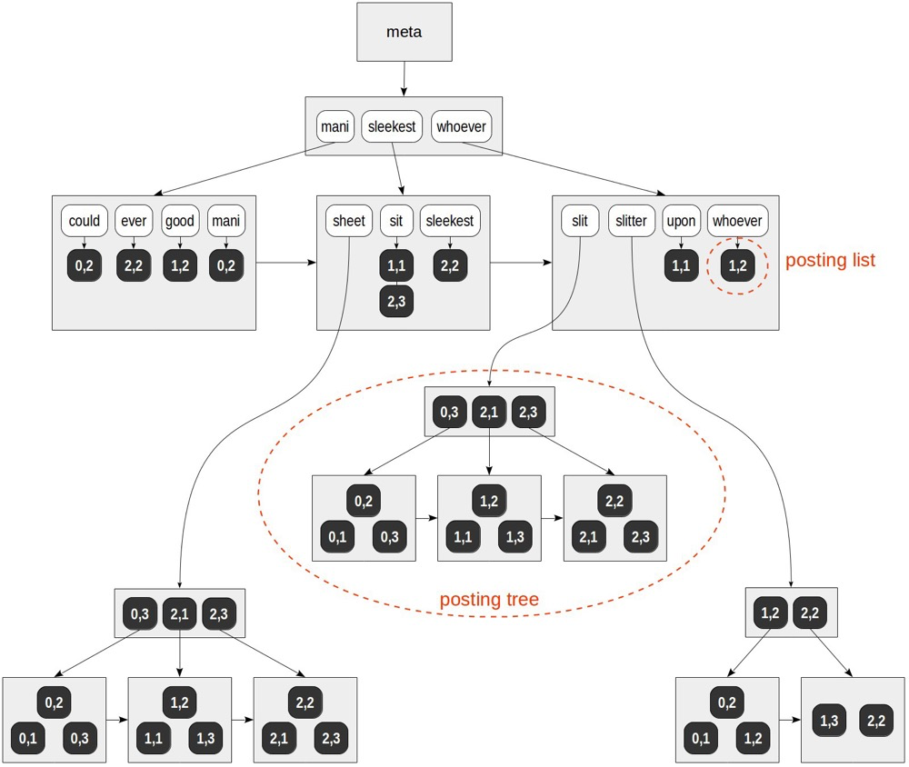
(https://postgrespro.com/blog/pgsql/4261647)
The index is sorted by token order, similar to BTREE; leaf nodes store ctids pointed to by tokens. Since the same token can come from multiple tuples, a token can point to multiple ctids. When multiple ctids exist, a posting tree is built — essentially a BTREE of ctids within.
Fulltext GIN addressing:
for “mani” — (0,2). for “slitter” — (0,1), (0,2), (1,2), (1,3), (2,2).
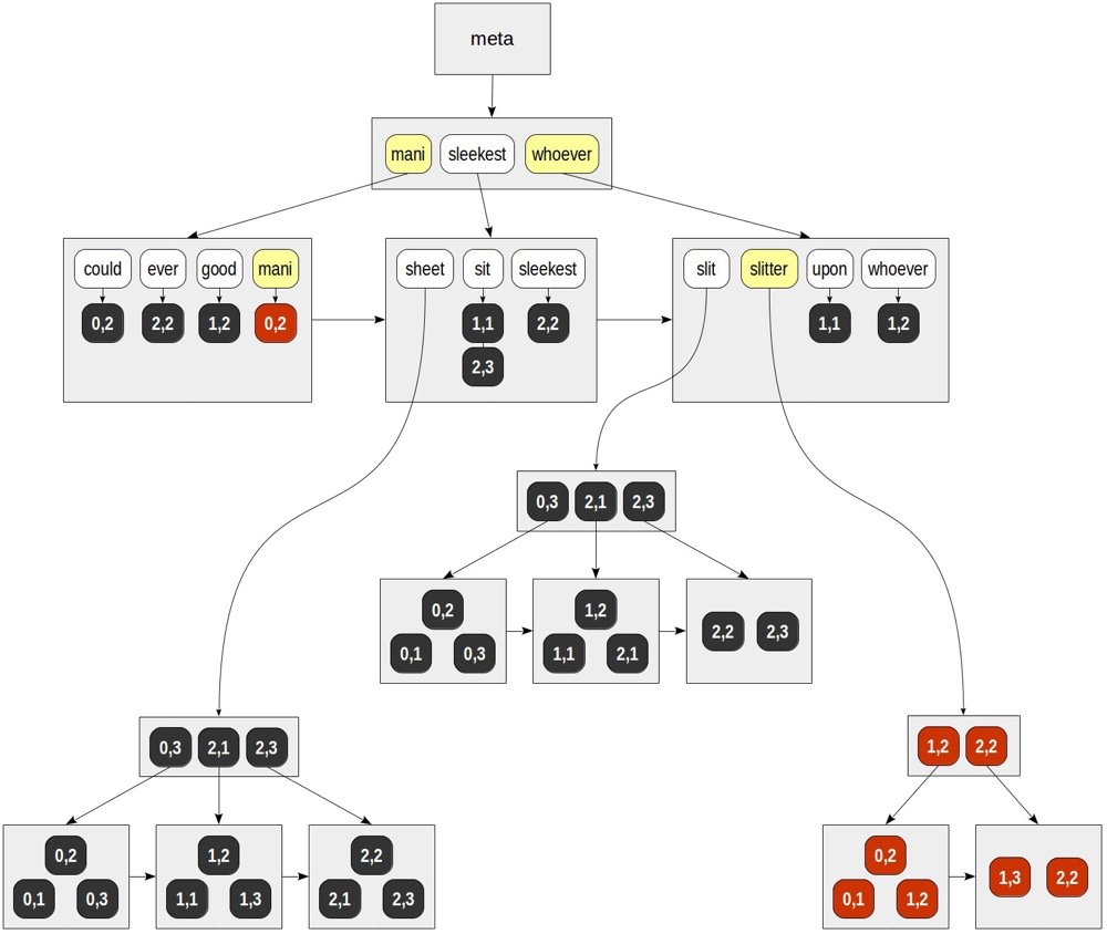
GIN updates:
Updating (insert/update/delete) a text generally requires updating many places in the GIN index because:
- One text can have many tokens scattered across GIN index branches
- One token may contain multiple ctids since many texts share that token
This makes GIN updates very expensive. Batch updates are typically better than row-by-row updates since some tokens are shared, reducing update work.
Besides batch updates, GIN provides fast update functionality (fastupdate = true):
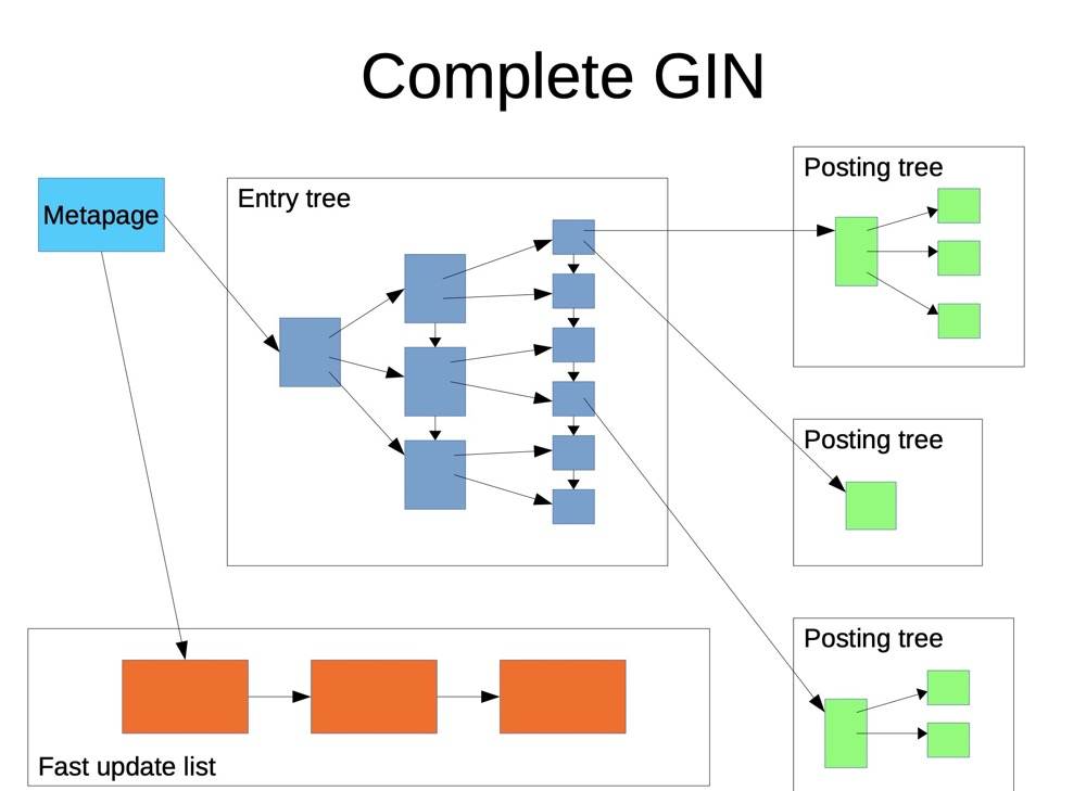
(https://www.pgcon.org/2016/schedule/attachments/434_Index-internals-PGCon2016.pdf)
GIN fast update:
- Incrementally updated data goes to a separate, unsorted area
- When vacuum runs or the list reaches
gin_pending_list_limit, incremental updates are written back to the main GIN index
GiST or GIN?
Both GiST and GIN are generalized index frameworks supporting full-text indexing, but their full-text index structures are completely different. GIST suits geographic and multi-dimensional spatial data; GIN mainly indexes scenarios where a key contains multiple values, such as arrays, full text, JSON.
- GIN indexes are faster than GiST; generally, full-text indexing can blindly choose GIN (reference: GIST vs GIN)
- Only with very frequent updates should GiST be considered, assuming fast update strategy can’t solve the update problem (e.g., configuring nightly write-back strategy). Better to compare GiST and GIN for various full-text indexing scenarios.
https://www.postgresql.org/docs/16/datatype-textsearch.html
https://postgrespro.com/blog/pgsql/4261647
(6) BRIN
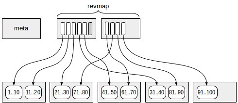
(https://postgrespro.com/blog/pgsql/5967830)
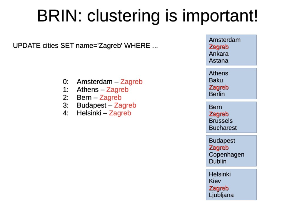
BRIN is not a tree-type index. Data is grouped in multiple pages (or blocks) as one range (similar to range partition but not physically partitioned). The table is divided into ranges, hence the name Block Range Index (BRIN).
The most critical BRIN component is the revmap layer, which stores only key value ranges and ctids, not the key values themselves. This is why BRIN indexes are very small — storing key values would make it like a branch-less BTREE.
Since only key value ranges and ctids are stored, data lookup requires accessing all data pages pointed to by matching revmap pages, then rechecking for final data rows.
															QUERY PLAN
----------------------------------------------------------------------------------
 Bitmap Heap Scan on flights_bi (actual time=75.151..192.210 rows=587353 loops=1)
   Recheck Cond: (airport_utc_offset = '08:00:00'::interval)
   Rows Removed by Index Recheck: 191318
   Heap Blocks: lossy=13380
   ->  Bitmap Index Scan on flights_bi_airport_utc_offset_idx
       (actual time=74.999..74.999 rows=133800 loops=1)
         Index Cond: (airport_utc_offset = '08:00:00'::interval)
Whether index key order matches storage order is critical. For example, non-sequentially stored extra key value data may be on “distant” pages, requiring extra IO to access distant data pages. Worst case, it may scan the entire table:
(https://www.pgcon.org/2016/schedule/attachments/434_Index-internals-PGCon2016.pdf)
BRIN suitable scenarios:
- BRIN indexes only suit data where index key order is highly consistent with storage order. Check the column’s correlation in pg_stats — should approach 1 (maybe -1 also works?), typically auto-increment primary keys and timestamp columns
- Nearly no update scenarios. Updates may reduce correlation
- BRIN indexes generally suit very large data, especially TB-scale and beyond
https://postgrespro.com/blog/pgsql/5967830
(7) RUM
RUM is an extension, not natively included in PG. RUM and GIN indexes are similar except RUM additionally stores tsvector position information.
Although GIN requires to_tsvector() (or direct tsvector) for tokenization, GIN doesn’t use the position information from to_tsvector(). For example, finding the distance between two tokens can’t be done with GIN — only via raw to_tsvector() data. RUM handles this.
RUM indexes attach token position information alongside ctids, compared to GIN:
(https://postgrespro.com/blog/pgsql/4262305)
RUM, similar to GIN, suits full-text indexing, with additional capabilities:
- Distance operators (e.g., <=>) for distance calculation
- Position-based sorting
https://postgrespro.com/blog/pgsql/4262305
(8) BLOOM
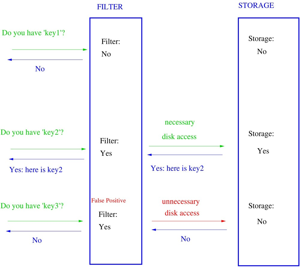
A Bloom filter quickly determines whether an element is in a set. Bloom filters can have false positives — “in set” isn’t guaranteed true, but “not in set” is guaranteed true. BLOOM indexes are also non-tree, flat structures (requiring recheck like BRIN).
(https://en.wikipedia.org/wiki/Bloom_filter)
Bloom indexes can index many columns. Similar to hash indexes, but unlike hash indexes, they can specify hashed fields and combine them, with total length limited by the length parameter. Because of the segmented hashing and truncation, false positives exist. Shorter length means higher false positive probability (max length 4096 bits).
create index on ... using bloom(...) with (length=..., col1=..., col2=..., ...);
(https://postgrespro.com/blog/pgsql/5967832)
https://www.postgresql.org/docs/current/bloom.html
https://postgrespro.com/blog/pgsql/5967832
Summary:
| Index Type | Structure | Operators | Access Complexity | Native? | Ordered? | Accurate? | Applicable Scenarios | Advantages | Disadvantages |
|---|---|---|---|---|---|---|---|---|---|
| btree | btree; branch stores key ranges, leaf nodes store keys and ctids, generally ascending | >=, =, IS NULL etc. common operators; leftmost prefix rule | O(logN) | Yes | Yes | Yes | High selectivity scenarios; not suitable for too-large data | Fits most scenarios; no extra sorting needed | Large key values make index very large; index fragmentation/splitting (HOT mitigates) |
| hash | Builds hash buckets; different hash values point to different rows | Only = | O(1) | Yes | No | Yes | Only = condition scenarios; large key values | Generally small; fast access | Very narrow use case |
| GiST | Index framework; R-TREE, RD-TREE; groups addresses at different layers for precision | Spatial operators: <-> distance, << left-of, @> contains etc. | Layer height | Yes | Yes (supports KNN) | Yes | GIS; KNN; frequently updated full-text index | GIS, multi-dimensional data | Special-case scenarios |
| sp-GiST/Q-tree | (sp-GiST is framework; index excludes overlapping data) Q-tree: each node has 4 internal nodes | Spatial operators: up/down/left/right, equality, contains | Layer height | Yes | Yes | Yes | GIS | GIS | GIS |
| sp-GiST/k-d tree | k-d tree: splits multi-dimensional space at nodes until no further split | Spatial operators | Min O(k), avg O(logN), max O(N/2) | Yes | Yes | Yes | GIS; multi-dimensional data | GIS, multi-dimensional data | Special-case scenarios |
| sp-GiST/radix-tree | radix-tree: each child synthesizes its parent | Common operators: =, >, ~ etc. | Min O(1), max O(N) | Yes | Yes | Yes | Scenarios without common data | Supports common operators beyond GIST | Limited scenarios; can be very slow |
| GIN | Index framework; similar to btree: branch stores token ranges, leaf stores tokens and ctids; one token pointing to multiple ctids may have sub-posting-tree; fast update enabled adds linked-list space for incremental data | Operators vary slightly by data type; generally @@ contains | Related to text length/token repetition; approx O(logN) | Yes | No (branches ordered but no token position info) | Yes | Key-contains-multiple-values scenarios: array, full text, JSON, many columns | Best choice for multi-value key scenarios | Updates need proper strategy |
| BRIN | Non-tree: groups data pages by range; rev index layer stores only key ranges and ctids | Common operators: < <= = >= > | Page lookup O(1); data return O(N), N=recheck rows | Yes | Not strictly ordered, only suits ordered data | No | Sequential storage (time-series, auto-increment); very large tables; nearly no updates; range queries | Very small index | Extremely demanding on correlation |
| RUM | Similar to GIN, but additionally stores token position info | Includes GIN operators plus position operators | Related to text length/token repetition; approx O(logN) | No | Yes (supports KNN lookup) | Yes | Key-contains-multiple-values scenarios; suitable for KNN | Stores position info beyond GIN | Requires extension installation |
| BLOOM | Each field hashed and truncated; non-tree, bitmap filtering | Common operators: < <= = >= > | Miss: O(1); hit: O(N), N=recheck rows | Yes | No | No | Suitable for miss scenarios | Can be very fast | Can be very slow on recheck |
Additional index section references:
Types of PostgreSQL Indexes. Short and clear
https://leopard.in.ua/2015/04/13/postgresql-indexes
https://pic.huodongjia.com/ganhuodocs/2017-07-15/1500104265.79.pdf
https://developer.aliyun.com/article/698090?spm=a2c6h.12873639.article-detail.43.702e7149IBMYL9
https://postgresql.us/events/pgopen2019/sessions/session/647/slides/45/look-it-up.pdf
https://www.pgcon.org/2016/schedule/attachments/434_Index-internals-PGCon2016.pdf
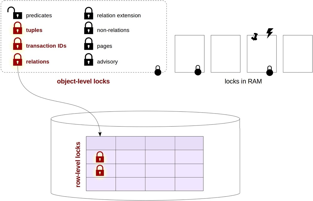
17. How Row Locks Are Implemented, Whether Stored in Shared Memory#
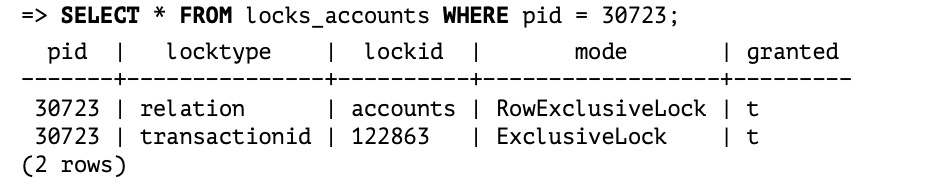
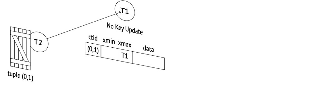
Row locks in PG are in the row header, not implemented in memory.
(1) After t1 updates without committing, it acquires exclusive locks on relation and transactionid:
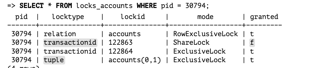
(2) t2 updating the same row gets blocked; this blocking is implemented via transactionid sharelock. t2 acquires both relation and tuple locks:
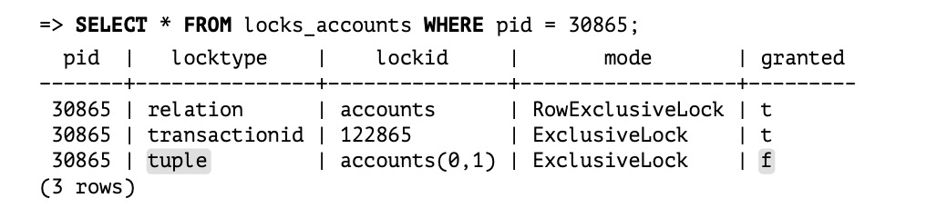
(3) t3 updating this row gets blocked via tuple exclusive lock:
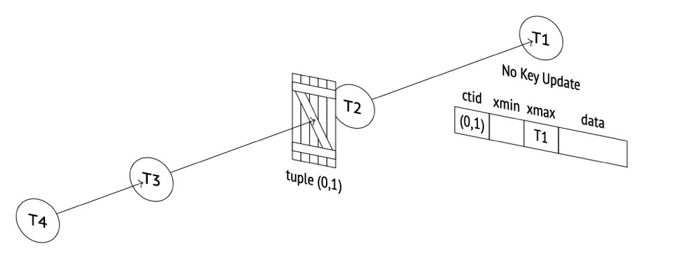
In summary, PG row locks are implemented jointly via transactionid locks, relation locks, and tuple locks:
《postgresql-internals-14》
https://postgrespro.com/blog/pgsql/5968005
18. Differences Between Streaming Replication and Logical Replication, and Their Applicable Scenarios#
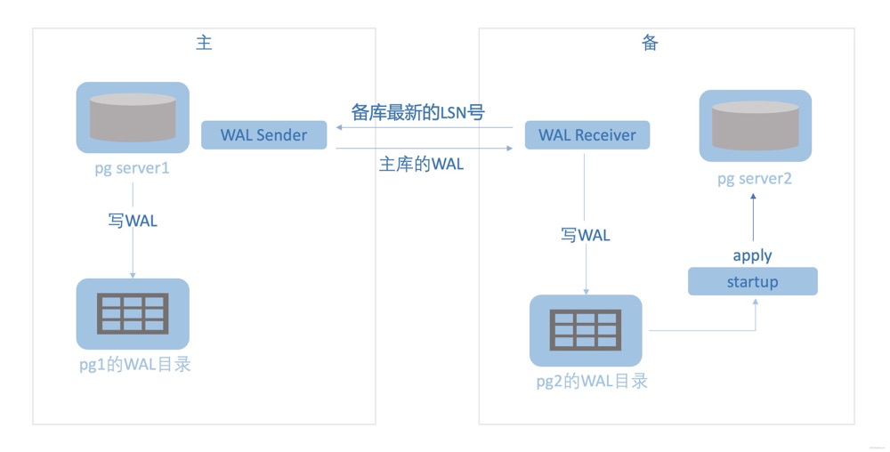
Streaming replication here generally refers to PG physical replication, synchronizing full WAL logs downstream for replay by the downstream PG instance at the physical block level:
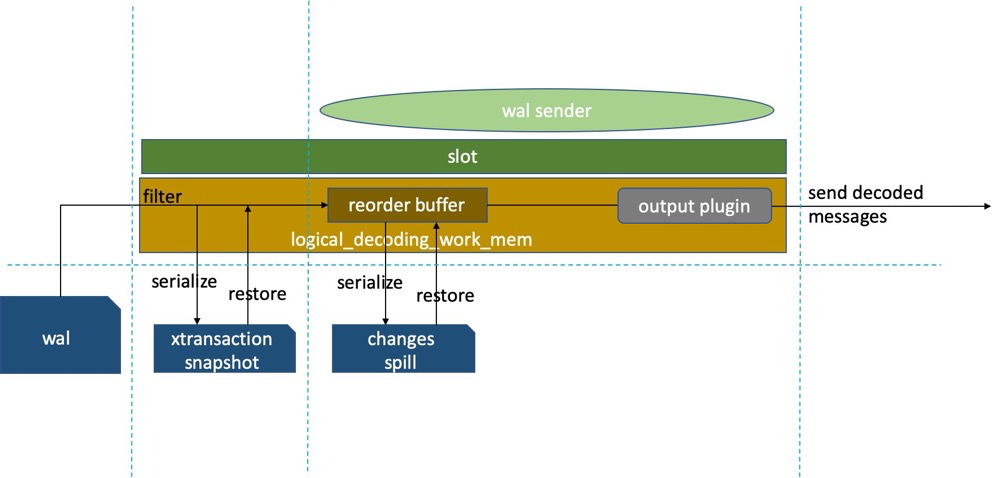
Logical replication requires logically decoding transaction information from WAL for relevant tables, ordering transactions via reorder buffer, then outputting data in the form determined by the output plugin. The downstream need not be a PG instance. Must have replication slots managing logical decoding, output plugin, reorder buffer, replication positions, etc., plus knowledge of replica identity, slot/sender status, and more:
Logical replication has many issues but is increasingly widely used and is a key focus area for PG community updates.
For example (incomplete list):
- logical_decoding_work_mem is no longer hardcoded 4096 (changes); it’s now a configurable GUC parameter. Decoding spill issues are somewhat mitigated
- PG14+ supports streaming logical replication: uncommitted transactions can transmit data downstream; subsequent commit info determines whether to apply the changes
- Standby servers support replication slots; logical replication can be established on standbys
- Failover slots (in progress?)
- Many more updates…
19. What Is Streaming Replication Conflict and Why It Occurs#
Cause of conflict:
The standby is running a query on a table (from application or manual connection). Meanwhile, the primary executes DROP TABLE, written to WAL and transmitted to the standby for replay. To ensure data consistency, PostgreSQL must rapidly replay WAL. The DROP TABLE and SELECT then conflict. Since the primary doesn’t know the standby’s transaction state, and the standby must stay consistent with the primary, “query conflict” occurs.
Conflict scenarios:
- Primary exclusive locks (including explicit LOCK commands and various DDL)
- Primary vacuum cleaning dead tuples — if the standby is using those tuples, conflict arises
- Primary drops a tablespace that the standby query is using
- Primary drops a database that the standby is using
Mitigating query conflicts (can’t fully resolve):
hot_standby_feedback: standby periodically notifies the primary of the minimum active transaction ID (xmin), preventing the primary vacuum from cleaning tuples older than the xmin value.
max_standby_streaming_delay: standby queries aren’t immediately canceled; instead wait for a period before throwing an error if not finished.
max_standby_archive_delay: waiting time before canceling standby queries due to conflicts from processing archived WAL logs.
vacuum_defer_cleanup_age: specifies how many transactions vacuum delays dead tuple cleanup by; i.e., vacuum and vacuum full won’t immediately clean just-deleted tuples.
20. PostgreSQL Permission System Overview#
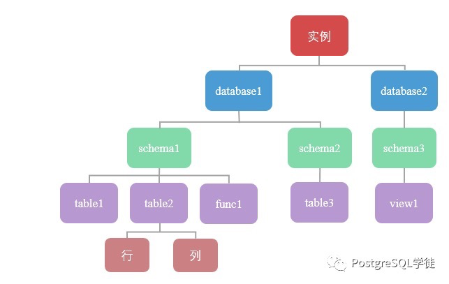
Hard to summarize comprehensively; it’s somewhat complex. Key points:
- Permission access requires each layer to be “open”; none can be missing
- Best to separate read-only/read-write/owner users
- Read-only and read-write permissions can be managed via roles
21. Common High Availability Solutions, Selection Criteria, Pros and Cons#
HA selection considerations:
- Sync mode choice, availability zones, cross-region multi-active
- Switchover, failover
- Load balancing, read/write separation
- Host, database, and application-level HA
- VIP switching, connection string HA, connection switching
- Solving single point of failure or split-brain; election mechanisms
Below are some known architectures:
pgpool-II+watchdog:
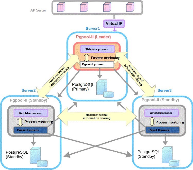
(https://www.pgpool.net/docs/latest/en/html/example-cluster.html)
Pros: automatic failover, read/write separation, load balancing, watchdog election Cons: complex configuration, pgpool doesn’t fully support all PG features, pgpool performance overhead, depends on watchdog election
patroni+etcd:
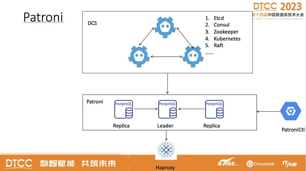
Pros: GUI (patroni), automatic failover, majority election Cons: learning curve, doesn’t support other databases (patroni)
patroni+pgbouncer+haproxy+etcd:
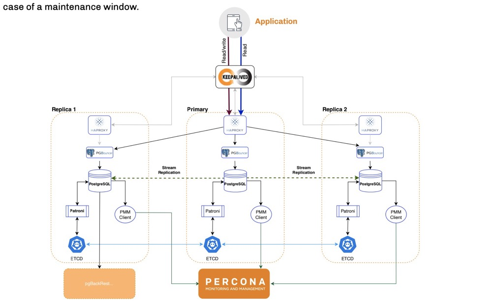
(https://www.percona.com/sites/default/files/eBook-PostgreSQL-High-Availability.pdf)
Pros: open-source stack: haproxy for load balancing, pgbouncer for connection pooling, patroni for cluster management, etcd for election Cons: very complex configuration
Ping An Financial Cloud rasesql architecture:
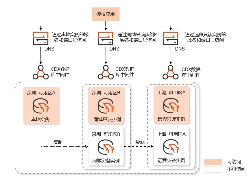
(https://www.ocftcloud.com/ssr/help/database/RASESQL/intro.Architecture)
Pros: failover support, simple architecture Cons: same-city remote can’t directly read-only access, higher resource usage, no election (?)
Alibaba Cloud Polar-X:
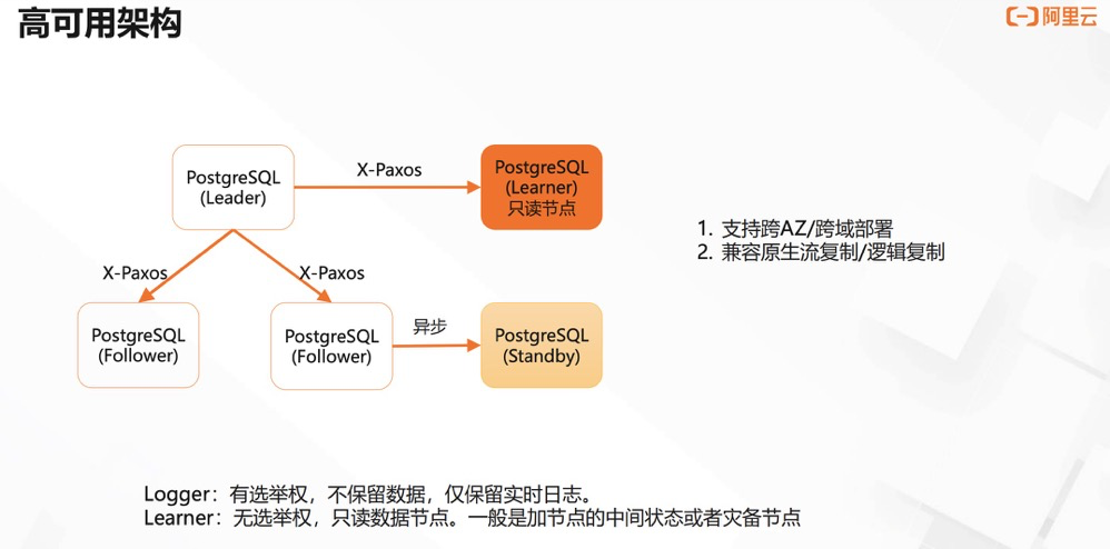
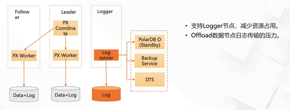
(PolarDB for PostgreSQL 三节点功能介绍)
Pros: read/write separation, can add non-voting nodes, failover, logger nodes participate in election/data flow/backup Cons: …
Google Cloud PG:
Three architecture options:
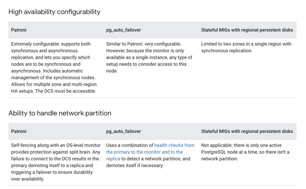
Google Cloud Native Architecture (MIG):
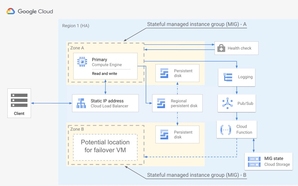
Pros: three options to choose from, well-documented! (the other two derive from open-source architectures with similar pros/cons; MIG cloud-native approach described below) MIG advantages: doesn’t depend on PG native HA; uses Regional persistent disk for data HA. Primary zone network isolation; disk can be attached to zone B in the same region (within 1 minute). MIG disadvantages: no read replicas; only within-region failover (no multi-region deployment)
Aurora for PG:
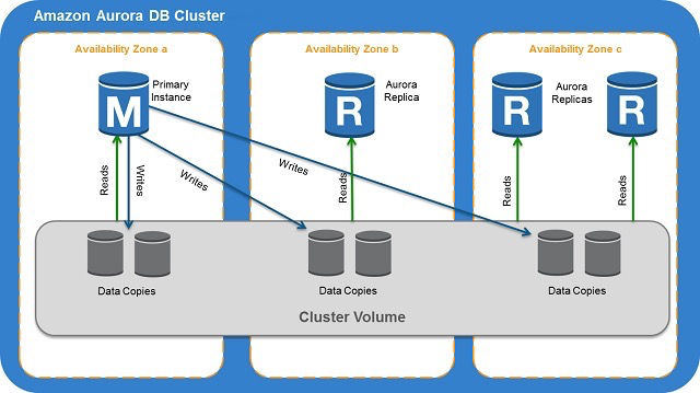
Pros: simple architecture, recovered primary node auto-joins cluster, multi-region deployment, standby readable Cons: (seemingly) no election mechanism; docs heavy on text, light on diagrams
崔健:PostgreSQL的高可以架构设计与实践
https://www.pgpool.net/docs/latest/en/html/example-cluster.html
使用Patroni和HAProxy创建高度可用的PostgreSQL集群
https://www.percona.com/sites/default/files/eBook-PostgreSQL-High-Availability.pdf
PolarDB for PostgreSQL 三节点功能介绍
https://docs.aws.amazon.com/AmazonRDS/latest/AuroraUserGuide/Aurora.Overview.html
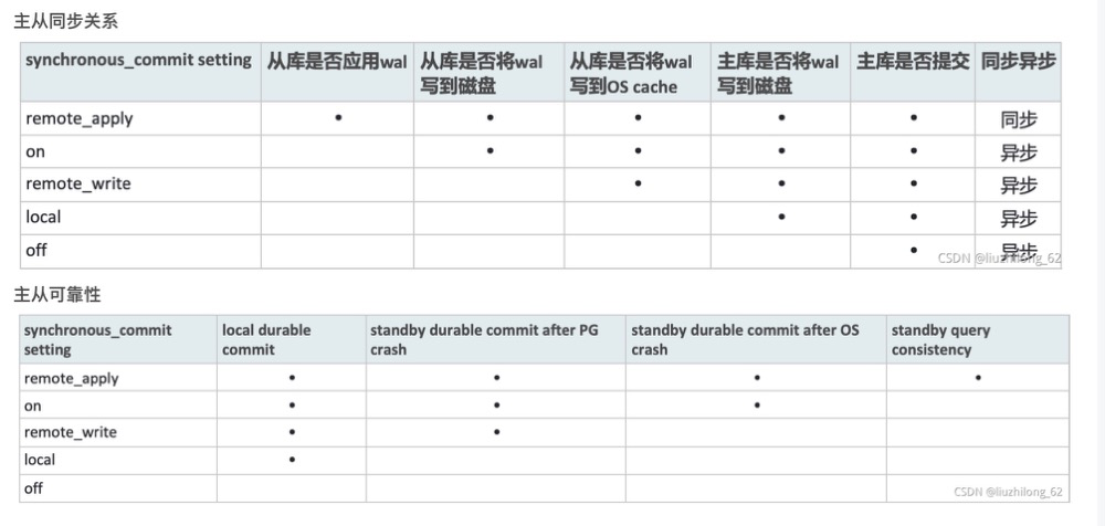
22. Five Levels of synchronous_commit; Why Standby Queries Can’t Immediately See Primary Inserts#
23. Transaction ID Wraparound Causes and Maintenance Optimization#
Why transaction ID wraparound exists:
Every non-query transaction consumes a transaction ID. Query transactions consume virtual transaction IDs (VXID), which are locally counted. Though VXID has wraparound issues, session restart resets VXID counting, so it’s rarely problematic.
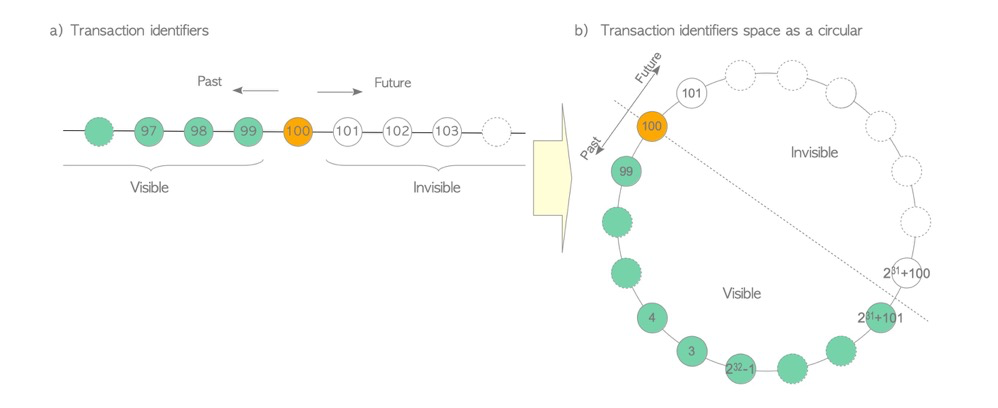
However, transaction IDs have an upper limit. TransactionId is a 32-bit unsigned integer, storing 2^32=4294967296 — about 4.2 billion transactions. At this point, transaction IDs must wrap around to the initial state, which is why transaction IDs form a ring.
Due to visibility rules, the 4.2 billion transactions must be split in half: one half represents the future, the other the past. The difference between max and min transactions in a PG instance cannot exceed 2.1 billion — hence the 2.1 billion transaction limit.
(https://www.interdb.jp/pg/pgsql05/01.html)
Transaction ID freezing:
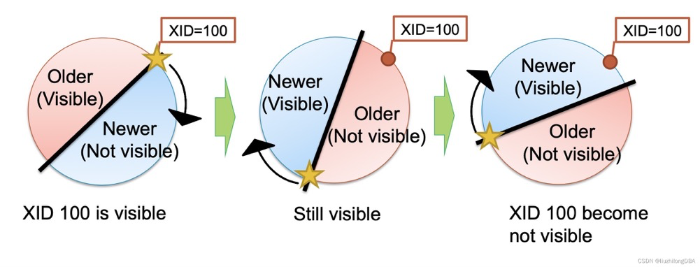
Due to visibility rules, if a visible row (e.g., xid=100) differs from the latest transaction by more than 2.1 billion, it becomes invisible:
(Forgot the source; look it up)
To solve this, the transaction ID freezing mechanism was introduced. Freezing sets the xmin of overly old tuples to FrozenXID=2, older than all normal transactions. That is, txid=2 is visible to all normal transactions (txid>=3). In version 9.4+, t_infomask’s xmin_frozen flag indicates frozen tuples rather than rewriting t_xmin to 2.
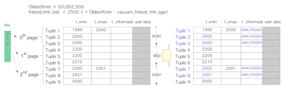
Lazy mode: The VM file was originally designed to reduce vacuum overhead by letting vacuum skip pages with no dead tuples (all-visible). Later (pg9.4), the freeze process was enhanced so lazy mode freezing can also skip all-visible pages during vacuum.
Lazy mode freeze trigger: triggered alongside vacuum operation (seems to have no independent trigger condition???)
Lazy mode freeze which tuples: except pages marked all-visible in VM that get skipped, freezes tuples whose xmin-to-active-transaction-ID (actually oldestxmin) gap exceeds vacuum_freeze_min_age (default 50M), marking them xmin_frozen. In the diagram below, tuple 9’s xmin=3000 won’t be frozen.
Lazy mode is more of a vacuum side-effect: since we’re already concurrently vacuum scanning and cleaning dead tuples with pages already scanned, we might as well freeze eligible tuples.
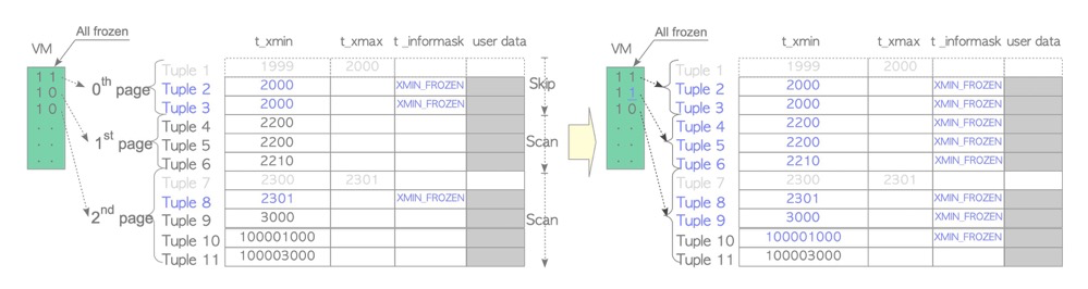
Eager mode: Lazy mode has a problem: it works alongside vacuum, skipping pages with no dead tuples (all-visible). If a page contains only live tuples (all-visible but not all-frozen) with very old xmin values, lazy mode alone can’t freeze them. So eager mode is needed: skip pages already marked all-frozen in VM and freeze the rest. In real scenarios, eager mode is typically the one running periodically and requiring attention: even if only one page in a table has tuples that are all inserts (even just one static page), eager mode is needed.
Eager mode freeze triggers:
Vacuum_freeze_table_agefor vacuum operations: when the database-level minimum xmin (actuallypg_database.datfrozenxid, also the minimum of allpg_class.relfrozenxidin that database) and the active transaction ID (actually oldestxmin) gap exceedsVacuum_freeze_table_age(default 150M), vacuum triggers eager mode freezing.autovacuum_freeze_max_agefor autovacuum: whether lazy mode or eager modeVacuum_freeze_table_age, vacuum must first be triggered. Relying solely on vacuum’s own trigger conditions for freezing is unreliable; a freeze-specific deadline parameter is needed:autovacuum_freeze_max_age. When tuple age exceedsautovacuum_freeze_max_age(200M), autovacuum is force-triggered for freezing. Even if autovacuum is disabled, this deadline-triggered freeze still works.
Eager mode freeze which tuples: similar to lazy mode, except for all-frozen pages (lazy uses all-visible — different), freezes tuples whose xmin-to-active-transaction-ID gap exceeds vacuum_freeze_min_age (default 50M). In the diagram, tuple 11 is not frozen.
vacuum freeze command: VACUUM FREEZE is equivalent to setting vacuum_freeze_min_age and vacuum_freeze_table_age to 0, performing eager mode freezing for all inactive xmin tuples.
vacuum_failsafe_age: Since large table vacuum operations are very slow, freeze may not finish before transaction ID wraparound occurs. Because freeze is done by the vacuum process, and vacuum has many other operations and parameter settings, to accelerate freeze, cost-based vacuuming, buffer strategy, and index vacuuming are all ignored. Parameter default is 1.6B; actually, during vacuum the effective value is no lower than autovacuum_freeze_max_age * 105%.
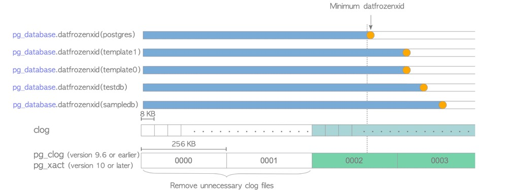
CLOG may also be updated: Additionally, if freezing updates pg_database.datfrozenxid, unnecessary CLOG is also cleaned. CLOG records transaction status for determining “relatively new” transaction and tuple visibility. If a database’s frozenxid has been advanced recently, meaning those “old” tuples have been marked as frozen — always visible — then “old” transaction status info in CLOG can be discarded.
Maintenance optimization: (summarized from Can Zong’s summary)
- Monitor pg_database.frozenxid in production. When approaching trigger values, proactively run VACUUM FREEZE during low-traffic windows rather than waiting for passive database triggers.
- Partition tables; overly large tables cause long prevent-wraparound operations
- Set different vacuum ages for large tables: ALTER TABLE test SET (autovacuum_freeze_max_age=xxxx);
- User-scheduled freeze: during low-traffic windows, VACUUM FREEZE large, aged tables
- Watch for freeze-blocking scenarios: long transactions, replication slots, hot_standby_feedback, pg_dump, cursors, orphan transactions
- Set sufficient worker processes to avoid vacuum scenarios queuing
- If load is a concern, consider enabling cost-based vacuuming (vacuum_cost_delay etc.)
- autovacuum_freeze_max_age should exceed vacuum_freeze_table_age to leave room for manual vacuum. Official recommendation: vacuum_freeze_table_age = 0.95 * autovacuum_freeze_max_age; if vacuum_freeze_table_age is below 0.95 * autovacuum_freeze_max_age, vacuum still takes 0.95 * autovacuum_freeze_max_age.
- vacuum_failsafe_age: PG14+ set reasonable vacuum_failsafe_age to accelerate large table freeze and prevent wraparound; should exceed autovacuum_freeze_max_age * 105%.
https://www.postgresql.org/docs/16/routine-vacuuming.html#VACUUM-FOR-WRAPAROUND
24. Vacuum / Autovacuum Functions and Tuning#
Functions:
- Clean up “dead tuples” left by UPDATE or DELETE operations
- Track available space in table blocks, update free space map
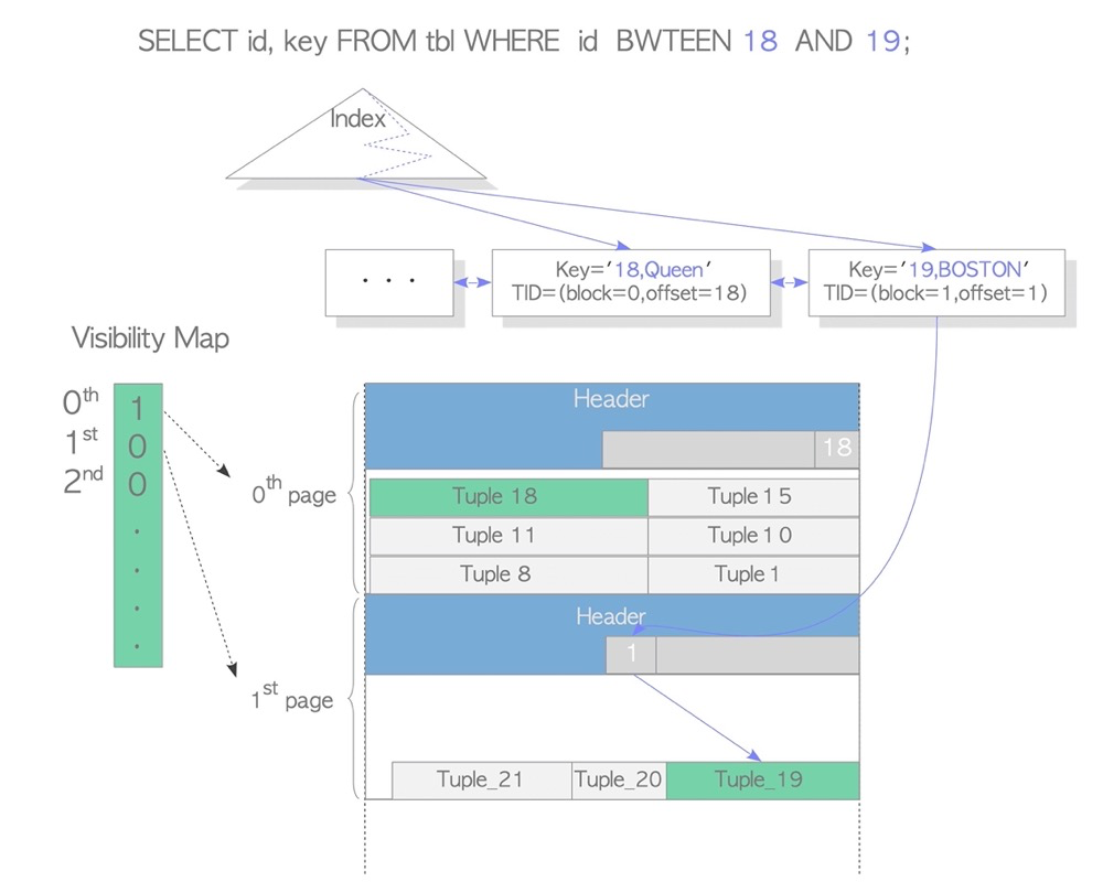
- Update visibility map needed for index-only scans
- “Freeze” rows in tables to prevent transaction ID wraparound
- Periodically ANALYZE to update statistics
Tuning:
- Set sufficient worker processes to avoid vacuum queuing
- Increase maintenance_work_mem (or autovacuum_work_mem)
- Watch for vacuum-blocking scenarios: long transactions, replication slots, hot_standby_feedback, pg_dump, cursors, orphan transactions
- For special tables (business-sensitive, large), set separate autovacuum trigger thresholds (threshold, fillfactor; insert threshold, fillfactor): dead tuple cleanup threshold, stats update threshold, wraparound prevention threshold
- For special tables, disable per-table autovacuum and run vacuum during off-peak hours for dead tuple cleanup, statistics, and wraparound
- If business load is a concern, enable cost-based vacuuming with sleep at thresholds
- Partition tables to avoid vacuum running endlessly or restarting immediately after finishing
- Avoid VACUUM FULL (8-level lock). Use logical replication + rename or pg_repack for table/index bloat handling, improving efficiency and reclaiming space
25. Function Volatility Categories and Why Functions Need EXECUTE#
VOLATILE (unstable, default):
- Can do anything, including modifying the database
- Within the same transaction, even with identical parameters, may return different results
- Obtains a snapshot for each query execution within the function, so even identical interactive queries within the same function may produce different results due to changing visible data
- Since recalculation is needed each time, the optimizer can’t pre-estimate; performance may be poor
- Function indexes not supported
- Typical functions: timeofday(), random(), all modifying functions
STABLE:
- Cannot modify the database
- Within the same transaction, identical parameters return identical results. Snapshot obtained at function start; internal queries don’t re-obtain; identical interactive queries within the function produce consistent results
- Function indexes not supported
- Typical functions: current_timestamp family; regardless of how many times called within a transaction, only one value
IMMUTABLE (very stable):
- Cannot modify the database
- Given identical parameters, always returns identical results. Snapshot acquisition principle same as STABLE
- Key difference from STABLE: IMMUTABLE not only caches the plan but reuses this plan in subsequent executions
- Function indexes supported
- Some database-parameter-dependent functions shouldn’t be marked IMMUTABLE, e.g., timezone-related functions should be STABLE
- Typical function: calculating 1+2
Why functions need EXECUTE:
PREPARE: parsed, analyzed, and rewritten
EXECUTE: planned and executed
Forcing SQL hard parsing: prevents SQL from using incorrect execution plans due to data skew.
Unlike plain SQL, plpgsql defaults to Plan Caching, automatically executing SQL as PREPARE, attempting to generate and cache generic plans for soft parsing. However, with data skew, cached execution plans may be inefficient and unacceptable for core business. In such cases, consider using EXECUTE statements to force per-variable-value execution plans, improving accuracy.
https://blog.csdn.net/Hehuyi_In/article/details/128885660
https://www.postgresql.org/docs/16/xfunc-volatility.html
26. Why Use CREATE INDEX CONCURRENTLY and Its Hazards#
Why CIC:
CREATE INDEX requires a ShareLock, which conflicts with DML’s RowExclusiveLock. So online business shouldn’t directly use CREATE INDEX. CIC uses ShareUpdateExclusiveLock, which doesn’t conflict with DML locks, so CIC is recommended for index creation.
CIC process:
- Insert index metadata into system catalogs (pg_class, pg_index), then open two transactions for two scans
- Open transaction 1, get snapshot1
- Before scanning table, wait for all transactions that modified the table (insert/delete/update) to finish
- Scan table and build index
- End transaction 1
- Open transaction 2, get snapshot2
- Before second scan, wait for all transactions that modified the table to finish
- DML on the table from transactions started after snapshot2 will update this index
- Second table scan, update index (version numbers from tuples allow identifying records changed between snapshot1 and snapshot2, merging them into the index)
- After index update, wait for transactions holding snapshots that started before transaction 2 to finish
- End index creation. Index becomes visible.
CIC issues:
- Opens two transactions sequentially, scanning the table one extra time vs CREATE INDEX
- Must wait for long transactions to finish before scanning can begin
- CIC-created indexes may become invalid
- CIC interrupted abnormally leaves an invalid index
- During CIC unique index creation, inserted/updated data violating unique constraints also causes CIC failure leaving an invalid index
- Invalid indexes still get updated by DML
- Partition parent tables don’t support CIC index creation; create indexes with CIC on child partitions one by one, then create the index on the parent with ONLY
27. HOT Principle#
HOT:
Without HOT, every tuple update would update indexes. Below, one additional updated tuple adds one index entry, and the old index entry points to the dead tuple. This causes index update, index space, and index vacuum pressure.
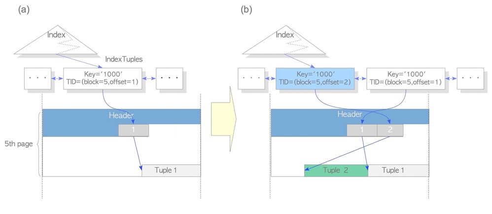
With HOT, in-page updates only update the tuple, not the index:
HOT tuples correspond to HEAP_HOT_UPDATED and HEAP_ONLY_TUPLE bits in infomask:
lzldb=> create table tt(a int);
lzldb=> create index idxtt on tt(a);
lzldb=> insert into tt values(1);
lzldb=> update tt set a=1; -- execute multiple times
lzldb=> select * from tt; -- after update, run a visibility check to write remaining clog commit info to tuple header

lzldb=> SELECT lp,case lp_flags when 0 then '0:LP_UNUSED' when 1 then 'LP_NORMAL' when 2 then 'LP_REDIRECT'  when 3 then 'LP_DEAD' end as lp_flags,
      t_ctid, raw_flags, combined_flags
         FROM heap_page_items(get_raw_page('tt', 0)),
          LATERAL heap_tuple_infomask_flags(t_infomask, t_infomask2)
         WHERE t_infomask IS NOT NULL OR t_infomask2 IS NOT NULL;
 lp | lp_flags  | t_ctid |                                        raw_flags                                        | combined_flags
----+-----------+--------+-----------------------------------------------------------------------------------------+----------------
  1 | LP_NORMAL | (0,2)  | {HEAP_XMIN_COMMITTED,HEAP_XMAX_COMMITTED,HEAP_HOT_UPDATED}                              | {}
  2 | LP_NORMAL | (0,3)  | {HEAP_XMIN_COMMITTED,HEAP_XMAX_COMMITTED,HEAP_UPDATED,HEAP_HOT_UPDATED,HEAP_ONLY_TUPLE} | {}
  3 | LP_NORMAL | (0,4)  | {HEAP_XMIN_COMMITTED,HEAP_XMAX_COMMITTED,HEAP_UPDATED,HEAP_HOT_UPDATED,HEAP_ONLY_TUPLE} | {}
  4 | LP_NORMAL | (0,5)  | {HEAP_XMIN_COMMITTED,HEAP_XMAX_COMMITTED,HEAP_UPDATED,HEAP_HOT_UPDATED,HEAP_ONLY_TUPLE} | {}
  5 | LP_NORMAL | (0,5)  | {HEAP_XMIN_COMMITTED,HEAP_XMAX_INVALID,HEAP_UPDATED,HEAP_ONLY_TUPLE}                    | {}
lp(line pointer)=1’s tuple points to row 2 via ctid(0,2); row 2 points to row 3… ultimately to row 5. ctid forms a chain pointing to the final data row. Dead tuples all carry HEAP_HOT_UPDATED, indicating the tuple is an updated row on the HOT chain; the chain tail has HEAP_ONLY_TUPLE, marking the end of the HOT chain.
With HOT, vacuum only cleans dead tuples within the page without updating indexes:
lzldb=> vacuum tt;
VACUUM
lzldb=> SELECT lp,case lp_flags when 0 then '0:LP_UNUSED' when 1 then 'LP_NORMAL' when 2 then 'LP_REDIRECT'  when 3 then 'LP_DEAD' end as lp_flags,
      t_ctid, raw_flags, combined_flags
         FROM heap_page_items(get_raw_page('tt', 0)),
          LATERAL heap_tuple_infomask_flags(t_infomask, t_infomask2)
         WHERE t_infomask IS NOT NULL OR t_infomask2 IS NOT NULL;
 lp | lp_flags  | t_ctid |                              raw_flags                               | combined_flags
----+-----------+--------+----------------------------------------------------------------------+----------------
  5 | LP_NORMAL | (0,5)  | {HEAP_XMIN_COMMITTED,HEAP_XMAX_INVALID,HEAP_UPDATED,HEAP_ONLY_TUPLE} | {}
After vacuum, dead tuples are cleaned.
On subsequent updates, a new HOT chain begins:
 lzldb=> update tt set a=1;
 lzldb=> update tt set a=1;
 lzldb=> select * from tt;
 lzldb=> SELECT lp,case lp_flags when 0 then '0:LP_UNUSED' when 1 then 'LP_NORMAL' when 2 then 'LP_REDIRECT'  when 3 then 'LP_DEAD' end as lp_flags,
      t_ctid, raw_flags, combined_flags
         FROM heap_page_items(get_raw_page('tt', 0)),
          LATERAL heap_tuple_infomask_flags(t_infomask, t_infomask2)
         WHERE t_infomask IS NOT NULL OR t_infomask2 IS NOT NULL;
 lp | lp_flags  | t_ctid |                                        raw_flags                                        | combined_flags
----+-----------+--------+-----------------------------------------------------------------------------------------+----------------
  2 | LP_NORMAL | (0,3)  | {HEAP_XMIN_COMMITTED,HEAP_XMAX_COMMITTED,HEAP_UPDATED,HEAP_HOT_UPDATED,HEAP_ONLY_TUPLE} | {}
  3 | LP_NORMAL | (0,3)  | {HEAP_XMIN_COMMITTED,HEAP_XMAX_INVALID,HEAP_UPDATED,HEAP_ONLY_TUPLE}                    | {}
  5 | LP_NORMAL | (0,2)  | {HEAP_XMIN_COMMITTED,HEAP_XMAX_COMMITTED,HEAP_UPDATED,HEAP_HOT_UPDATED,HEAP_ONLY_TUPLE} | {}
Why doesn’t the new HOT chain start from lp1? Because lp1 is already occupied — the index still points to lp1.
lzldb=> SELECT itemoffset, ctid, data, dead, htid, tids[0:2] AS some_tids
         FROM bt_page_items('idxtt',1);
 itemoffset | ctid  |          data           | dead | htid  | some_tids
------------+-------+-------------------------+------+-------+-----------
          1 | (0,1) | 01 00 00 00 00 00 00 00 | f    | (0,1) |
htid (0,1) is page 0, lp 1. Vacuum only cleaned the data page; the index was not updated. Vacuum only cleaned dead tuples and the middle of the HOT chain; HOT chain head and tail ctids were untouched.
INDEX ONLY SCAN:
Index-only scan is a common and efficient scan method across databases: it returns results by accessing only index pages without touching data pages. However, this is problematic in PG because visibility information is stored in data page headers, not index pages. Accessing only the index can’t support MVCC in principle.
The VM file not only supports vacuum skipping all-visible pages but also supports INDEX ONLY SCAN for visibility determination on all-visible pages:
Reference: interdb
28. Does PostgreSQL Have Lock Escalation?#
Basically no.
Only Predicate lock has escalation. Predicate lock is used when serializable isolation is needed, intended to lock predicates and prevent data anomalies to achieve serializability. In PG, this corresponds to SIReadLock.
- Predicate lock’s finest granularity is locking rows within a range
- When row count exceeds a threshold, lock the corresponding page
- When page count exceeds a threshold, lock the corresponding table
- Predicate lock has only 3 lock levels: row, page, table
https://postgrespro.com/blog/pgsql/5968020
29. Replication Slot Functions and Hazards#
For physical replication, replication slots aren’t strictly necessary; hot_standby_feedback and other parameters can manage WAL. With replication slots, those parameters become unnecessary — slots manage WAL logs.
For logical replication, replication slots are mandatory; one logical replication link corresponds to one slot. For logical replication, slots manage not only WAL logs but also logical decoding, output plugin, decoding/sending positions (LSN), allowing retransmission of decoded logs after replication interruption.

Replication slot hazards:
Actually, replication slots have no inherent hazards. Their primary function is simplifying WAL log management. Without slots, you still need WAL management strategies. The PG community recommends using slots. Just note: always clean up unused slots to prevent them holding old positions that block WAL cleanup, filling the disk. Additionally, DBAs shouldn’t casually drop slots — once dropped, position info is lost, and downstream links may need data reinitialization and resynchronization. Better to confirm whether the replication link can restart syncing.
30. Why Deadlocks Occur and Deadlock Detection Mechanism#
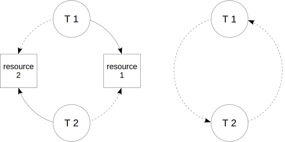
Simplest case: transaction T1 holds resource 1, transaction T2 holds resource 2. If T1 tries to acquire resource 2 and T2 tries to acquire resource 1, a deadlock forms. Without management, deadlocks can wait indefinitely, so all DBMS have deadlock detection. Deadlocks usually indicate business logic issues. If no explicit cancellation of one transaction in the “ring” breaks it, PG auto-detects deadlocks and force-terminates one transaction via the deadlock_timeout parameter (default 1s); other transactions in the “ring” can continue.
https://postgrespro.com/blog/pgsql/5968020
31. SQL Performance Troubleshooting Approaches#
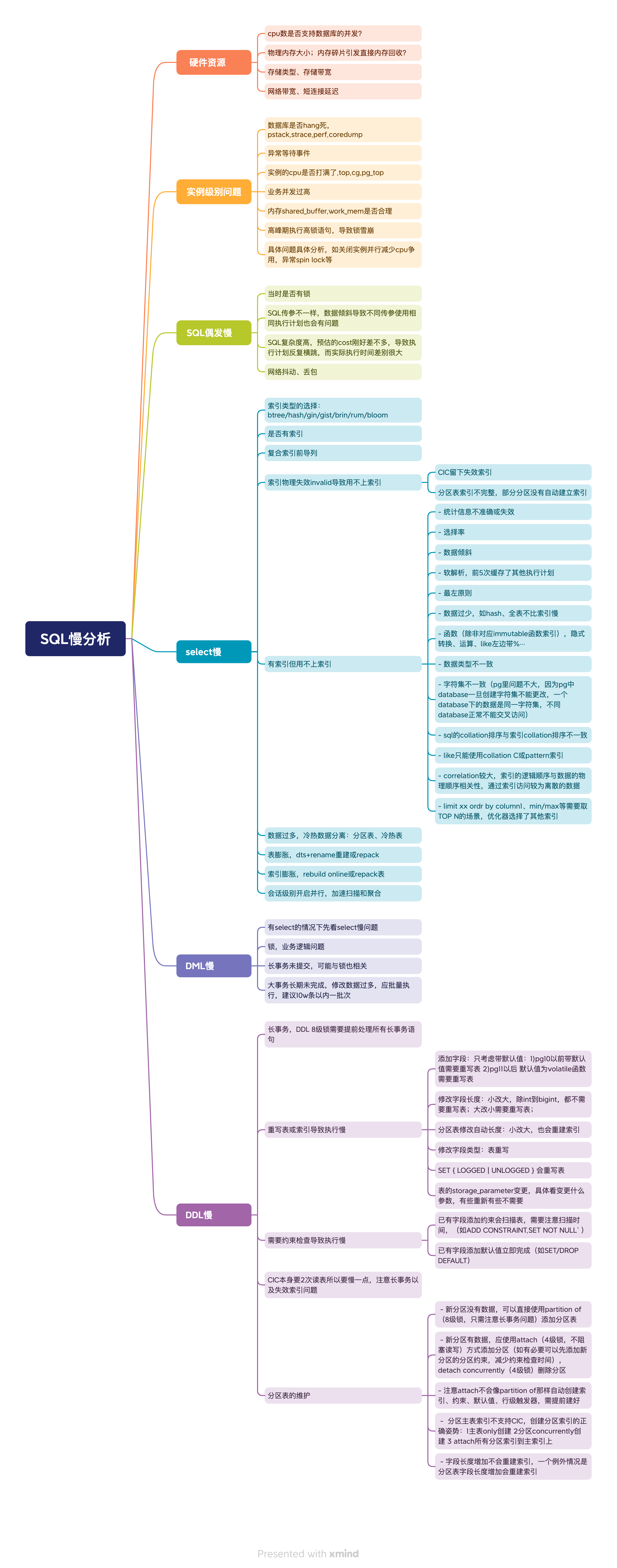
32. Why Use Partitioned Tables, Advantages and Disadvantages#
Partitioned tables split table data into smaller physical fragments to improve performance, availability, and manageability, transparent to applications. Partitioned tables are a common optimization for large tables in relational databases. DBMS generally provide partition management, and applications can directly access partitioned tables without architecture changes — though good performance requires proper partition access patterns.
PG natively supports declarative partitioning and inheritance partitioning. Common plugin-based implementations include pg_pathman. PG10 introduced declarative partitioning with many enhancements in subsequent versions (see PostgreSQL Partitioned Tables — History). PG12+ with declarative partitioning is recommended.
Advantages of partitioned tables:
- SQL performance improvement. In some scenarios, e.g., splitting large data into multiple partitions where SQL only queries one partition, partition pruning can dramatically improve performance
- Partitions work with indexes. Accessing one partition’s index is more efficient than accessing an unpartitioned large index
- Dropping a partition is more efficient than deleting many rows. Common in time-range partitioning: dropping an unused historical partition is very fast, while DELETE without partitions is slow and requires extra maintenance
- Faster vacuum. Vacuuming a large table for old version cleanup or statistics collection can be very slow; SQL problems may arise before vacuum finishes. With partitions, vacuum is much faster
- IO distribution. Different partitions can be placed on different paths/disks. Rarely used data can go on cheaper disks
- More maintenance techniques. Directly maintaining a huge table is very difficult (e.g., vacuuming an extremely large table has many issues), while partitioned table partitions can be vacuumed individually. Also, attach/detach, local indexes/constraints etc. can be flexibly used
- May enable partition-wise join or partition-wise aggregation features
Disadvantages of partitioned tables:
- In PG, partitions are also tables; too many tables cause slow parsing and large relcache metadata caching
- Too many tables may cause errors. Reference: 较少的分区也报错too many range table entries
- Even if partition count doesn’t error, without partition pruning during plan generation (may happen at execution), EXPLAIN output becomes very large, and logs become bloated with long plans
- Strange issues: 不同用户查看到不同的执行计划
Major limitations of PG native partitioned tables:
- No native automatic partition creation
- Only local indexes supported, no global indexes
- Primary key must include the partition key. PostgreSQL currently can only enforce uniqueness within individual partitions, hence this limitation. Oracle and MySQL don’t have this restriction
- Unique index must include the partition key (same reason as primary key)
- Cannot create global constraints (child tables inherit but can’t create table-level global constraints)
Partitioned table maintenance:
- New partitions without data: directly use PARTITION OF (8-level lock; just watch for long transactions)
- New partitions with data: use ATTACH (4-level lock, doesn’t block reads/writes) to add; if needed, pre-add partition constraints to reduce constraint check time. DETACH CONCURRENTLY (4-level lock) to remove partitions
- Note: ATTACH doesn’t auto-create indexes, constraints, defaults, or row-level triggers like PARTITION OF does; create them beforehand
- Partition parent table indexes don’t support CIC. Correct approach for partition index creation: 1) create ONLY on parent 2) create CONCURRENTLY on partitions 3) ATTACH all partition indexes to the parent; the index auto-marks as valid
- Increasing column length won’t rebuild indexes, EXCEPT for partitioned tables where it WILL rebuild indexes
33. Soft Parsing vs Hard Parsing Concepts#
Hard parsing: For a SQL statement, the optimizer must first perform lexical and syntax analysis, converting it into a query tree PG can understand, then rewrite and optimize it, generating an execution plan tree before the executor can execute. This full parsing process is called hard parsing.
Soft parsing: Obviously, performing such complex steps for every statement each time would be very inefficient. So PG caches SQL execution plans in process memory. When certain conditions are met, cached plans can be used directly, improving efficiency. This is soft parsing.
PG bind-variable SQL parsing: the five-time mechanism:
The five-time mechanism prevents data skew from causing inefficient execution plans.
First 5 executions: each generates an execution plan based on actual bound variables (called custom plans) — this is hard parsing. 6th execution: generates a generic execution plan (generic plan) and compares it with the previous 5 plans.
- If not worse than the first 5: the 6th plan is fixed; subsequently, regardless of parameter changes, the SQL execution plan won’t change — this is soft parsing
- If worse than any of the first 5 plans: every subsequent execution regenerates the plan — all hard parsing
Forcing soft/hard parsing:
PG 12 introduced the force_custom_plan parameter with options:
- auto: default, uses the five-time mechanism
- force_custom_plan: always hard parse; suitable for SQL with data skew where performance and stability are critical
- force_generic_plan: always use generic plan; suitable for SQL without data skew or where performance/stability requirements are lower
PG 14 added generic_plans and custom_plans columns to pg_prepared_statements, showing counts for both plan types. Since PG execution plans are only cached in-process, pg_prepared_statements only shows the current session’s SQL, not other sessions or global info.
Five-time mechanism source code:
/*
 * choose_custom_plan: choose whether to use custom or generic plan
 *
 * This defines the policy followed by GetCachedPlan.
 */
static bool
choose_custom_plan(CachedPlanSource *plansource, ParamListInfo boundParams)
{
	double		avg_custom_cost;

...

	/* Let settings force the decision */
	if (plan_cache_mode == PLAN_CACHE_MODE_FORCE_GENERIC_PLAN)
		return false;
	if (plan_cache_mode == PLAN_CACHE_MODE_FORCE_CUSTOM_PLAN)
		return true;

	/* See if caller wants to force the decision */
	if (plansource->cursor_options & CURSOR_OPT_GENERIC_PLAN)
		return false;
	if (plansource->cursor_options & CURSOR_OPT_CUSTOM_PLAN)
		return true;

	/* Generate custom plans until we have done at least 5 (arbitrary) */
	if (plansource->num_custom_plans < 5)
		return true;

	avg_custom_cost = plansource->total_custom_cost / plansource->num_custom_plans;

	/*
	 * Prefer generic plan if it's less expensive than the average custom
	 * plan.  (Because we include a charge for cost of planning in the
	 * custom-plan costs, this means the generic plan only has to be less
	 * expensive than the execution cost plus replan cost of the custom
	 * plans.)
	 *
	 * Note that if generic_cost is -1 (indicating we've not yet determined
	 * the generic plan cost), we'll always prefer generic at this point.
	 */
	if (plansource->generic_cost < avg_custom_cost)
		return false;

	return true;
}34. What Are VM / FSM / INIT Files#
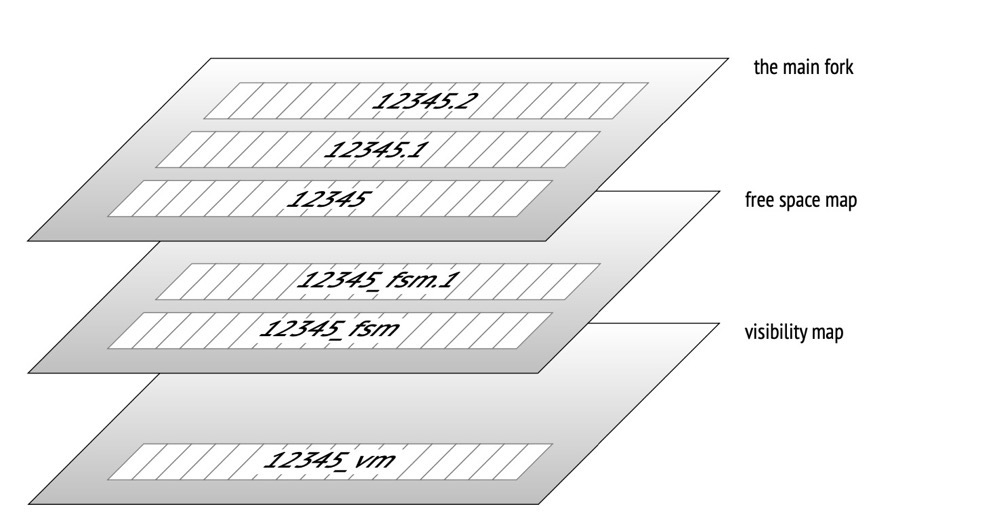
Numeric suffix: Files fork when exceeding 1GB (default); changeable at build time via ./configure --with-segsize
VM: Visibility map, containing all-visible and all-frozen info. Helps: 1) accelerate vacuum scanning (skip all-visible pages) 2) accelerate eager freeze (skip all-frozen pages) 3) support INDEX ONLY SCAN (all-visible pages don’t need page access for tuple visibility checks)
FSM: Free space map, helping PG locate free space on pages. For index pages, since indexes are ordered, recording per-page free space is less meaningful; index FSM files only contain fully empty index pages.
INIT: A fork file only for unlogged tables, size 0, marking the data file as unlogged.
《postgresql-internals-14》
35. Memory Reclaim Mechanisms: kswapd / Direct Memory Reclaim / pdflush#
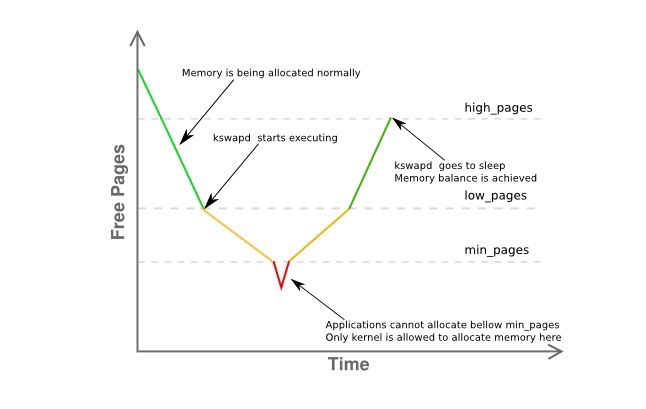
Memory reclaim mechanisms:
Background memory reclaim (kswapd): When physical memory is tight, the kswapd kernel thread is woken to reclaim memory asynchronously, not blocking process execution. Direct memory reclaim: If background async reclaim can’t keep up with process memory allocation requests, direct reclaim begins — synchronous, blocking process execution.
(https://vivani.net/2022/06/14/linux-kernel-tuning-page-allocation-failure/)
pages_low: When available free pages drop below pages_low, buddy allocator wakes kswapd; kernel begins swapping pages to disk. pages_min: When available pages reach pages_min, page reclaim pressure is high because the memory zone urgently needs free pages. Allocator performs kswapd work synchronously — sometimes called direct reclaim. pages_high: Once kswapd is woken and releasing pages, only when available pages reach pages_high does the kernel consider the zone “balanced”. At pages_high, kswapd re-enters sleep. Free pages above pages_high mean the zone state is ideal. Memory reclaim operates per-zone; /proc/zoneinfo shows min, low, high values.
vm.min_free_kbytes (the min_pages line) is a critically important OS parameter. Very low values prevent effective system memory reclamation, potentially causing crashes and service interruptions. Excessively high values increase reclaim activity, causing allocation latency and potentially immediate out-of-memory states.
pdflush and kcompactd:
pdflush: pagecache dirty pages must be written to disk. Whether via sync (fsync etc.), OS-scheduled flushing, or database commits, ultimately the Linux kernel thread pdflush handles the flushing work.
kcompactd: page compaction specifically targets memory fragmentation cleanup (flushing also works since memory returns to the buddy system). Unlike pdflush flushing, memory compaction doesn’t require disk writes.
Observing memory reclaim:
sar is one of the most comprehensive Linux system performance analysis tools, reporting on multiple dimensions: file read/write, syscall usage, disk I/O, CPU efficiency, memory usage, process activity, and IPC.
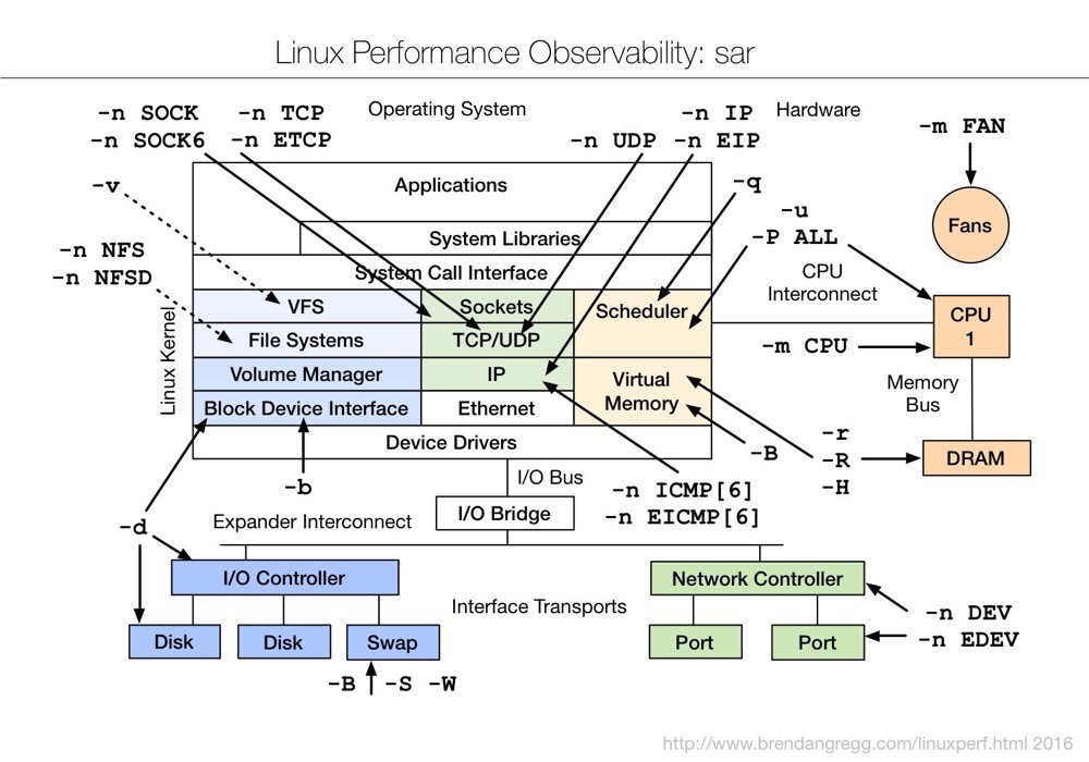
sar -B observes kswapd and direct memory reclaim:
Example: sar viewing memory page status
sar -B 1 3
- pgpgin/s: KB read from disk/SWAP into memory per second
- pgpgout/s: KB written from memory to disk/SWAP per second
- fault/s: page faults per second (major + minor)
- majflt/s: major page faults per second
- pgfree/s: pages placed in free queue per second
- pgscank/s: pages scanned by kswapd per second
- pgscand/s: pages directly scanned per second
- pgsteal/s: pages cleared from cache per second to meet memory needs
- %vmeff: percentage of stolen pages (pgsteal) vs total scanned (pgscank + pgscand)
Example: sar viewing historical memory info
sar -B -s "08:00:00" -e "10:00:00"
# Without -e means from start time to now
$ sar -B -s "08:00:00"
09:45:01 PM  pgpgin/s pgpgout/s   fault/s  majflt/s  pgfree/s pgscank/s pgscand/s pgsteal/s    %vmeff
09:46:01 PM 414429.37 395024.08 179478.63      0.07 352922.62  12003.78   4266.52  16269.42     99.99
09:47:01 PM 879907.08 337948.43 157970.97      0.02 402290.21      0.00      0.00      0.00      0.00
09:48:01 PM 772977.43 507343.30 150255.50      0.05 466742.08      0.00   5821.28   5821.27    100.00
Strong recommendation: linux内存浅析
36. Process Scheduling, D Process Hazards and Causes#
Not fully understanding what “process scheduling” specifically refers to here; I’ll answer in terms of IPC (Inter-Process Communication).
IPC:
Since user space in virtual address space can’t be accessed by other user processes, achieving multi-process user access to the same memory data via kernel space inevitably involves context switching (as shown on the right below). Multi-process applications clearly need inter-process access, so a method enabling user processes to directly access the same physical memory emerged: shared memory (as shown on the left below).
Shared memory is one IPC (Inter-Process Communication) mechanism; others include message queues and semaphores. Shared memory is one of the fastest IPC mechanisms because it doesn’t require inter-process data copying — processes access shared memory through their own address spaces.
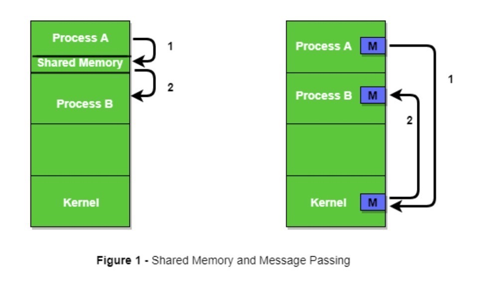
(https://www.geeksforgeeks.org/inter-process-communication-ipc/)
Shared memory has many implementations. In PG, shared_buffer defaults to mmap for shared memory (corresponds to shared_memory_type); parallel queries default to POSIX (corresponds to dynamic_shared_memory_type).
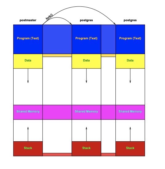
(https://momjian.us/main/writings/pgsql/inside_shmem.pdf)
D Process:
D process meaning: Uninterruptible sleep state. Indicates the process is waiting for an external event to complete, such as disk I/O or network requests. Normally, D processes cannot be directly terminated.
Causes of D processes: The process is waiting for an external event, typically direct memory reclaim — synchronous and blocking application disk access. At that moment, disk-access-related processes are in D state. Note: D processes are triggered at the OS or hardware level, largely unrelated to the application itself (a little). For example, a PG large query session itself won’t produce D processes and can be killed.
37. Packet Capture and Analysis of PostgreSQL Protocol#
PG supported protocols:
- Connection protocols:
- TCP/IP: PostgreSQL’s most common communication method, allowing client-server network connections and data exchange.
- Unix domain socket: For same-host client-server connections, faster than TCP/IP.
- SSL/TLS: PostgreSQL supports SSL/TLS encryption on TCP/IP connections for data transmission security. TLS is SSL’s successor; PG (seemingly) no longer supports SSL protocol itself, though related parameters remain for TLS use.
- Password authentication protocols:
- MD5: As the earlier default password authentication protocol, MD5 (Message Digest Algorithm 5) stores and verifies user passwords server-side.
- SCRAM-SHA-256: A more secure authentication protocol using SHA-256 hashing and challenge-response for user authentication. PG10+ gradually replaces MD5.
Simple packet capture analysis:
tcpdump capture command:
tcpdump tcp port 5432 -i lo -s0 -nSX -vvvCapture a count(*) (already connected to database via psql -h):
lzldb=> select count(*) from t1;  -- just capture this
 count
-------
     4
Captured content:
15:51:34.828820 IP (tos 0x0, ttl 64, id 29027, offset 0, flags [DF], proto TCP (6), length 82)
    172.18.10.85.37240 > 172.18.10.85.postgres: Flags [P.], cksum 0x6d13 (incorrect -> 0x57c6), seq 1091052893:1091052923, ack 3014367256, win 350, options [nop,nop,TS val 92480460 ecr 92427582], length 30
        0x0000:  4500 0052 7163 4000 4006 5c74 ac12 0a55  E..Rqc@.@.\t...U
        0x0010:  ac12 0a55 9178 1538 4108 255d b3ab 9818  ...U.x.8A.%]....
        0x0020:  8018 015e 6d13 0000 0101 080a 0583 23cc  ...^m.........#.
        0x0030:  0582 553e 5100 0000 1d73 656c 6563 7420  ..U>Q....select.
        0x0040:  636f 756e 7428 2a29 2066 726f 6d20 7431  count(*).from.t1
        0x0050:  3b00                                     ;.
15:51:34.830090 IP (tos 0x0, ttl 64, id 49370, offset 0, flags [DF], proto TCP (6), length 115)
    172.18.10.85.postgres > 172.18.10.85.37240: Flags [P.], cksum 0x6d34 (incorrect -> 0x6e5c), seq 3014367256:3014367319, ack 1091052923, win 342, options [nop,nop,TS val 92480461 ecr 92480460], length 63
        0x0000:  4500 0073 c0da 4000 4006 0cdc ac12 0a55  E..s..@.@......U
        0x0010:  ac12 0a55 1538 9178 b3ab 9818 4108 257b  ...U.8.x....A.%{
        0x0020:  8018 0156 6d34 0000 0101 080a 0583 23cd  ...Vm4........#.
        0x0030:  0583 23cc 5400 0000 1e00 0163 6f75 6e74  ..#.T......count
        0x0040:  0000 0000 0000 0000 0000 1400 08ff ffff  ................
        0x0050:  ff00 0044 0000 000b 0001 0000 0001 3443  ...D..........4C
        0x0060:  0000 000d 5345 4c45 4354 2031 005a 0000  ....SELECT.1.Z..
        0x0070:  0005 49                                  ..I
15:51:34.830098 IP (tos 0x0, ttl 64, id 29028, offset 0, flags [DF], proto TCP (6), length 52)
    172.18.10.85.37240 > 172.18.10.85.postgres: Flags [.], cksum 0x6cf5 (incorrect -> 0x5cb9), seq 1091052923, ack 3014367319, win 350, options [nop,nop,TS val 92480461 ecr 92480461], length 0
        0x0000:  4500 0034 7164 4000 4006 5c91 ac12 0a55  E..4qd@.@.\....U
        0x0010:  ac12 0a55 9178 1538 4108 257b b3ab 9857  ...U.x.8A.%{...W
        0x0020:  8010 015e 6cf5 0000 0101 080a 0583 23cd  ...^l.........#.
        0x0030:  0583 23cd                                ..#.
Reading packets visually… simple analysis shows this count statement only generated 3 packets, and you can even see the select.count(*).from.t1 statement.
Wireshark packet analysis:
Window 1:
tcpdump tcp port 5432 -i lo -s0 -nSX -vvv -w tcpdump.capWindow 2:
[postgres@iZ2vcdugd3f2h0t7x20pqmZ data]$ psql -h 172.18.10.85  -p 5432 -d lzldb -U lzl  -- step 1, connect
Password for user lzl:    -- step 2, enter password
lzldb=> select count(*) from t1;  -- step 3, query
 count
-------
     4

lzldb=> \q   -- step 4, exit
Note 4 steps, corresponding to at least 4 packet sections:
- Step 1 - connection request
- Step 2 - password entry
- Step 3 - SQL query
- Step 4 - disconnect
Now analyze tcpdump.cap with Wireshark.
- Step 1 - Connection Request [1-10] — TCP three-way handshake [1-3]:
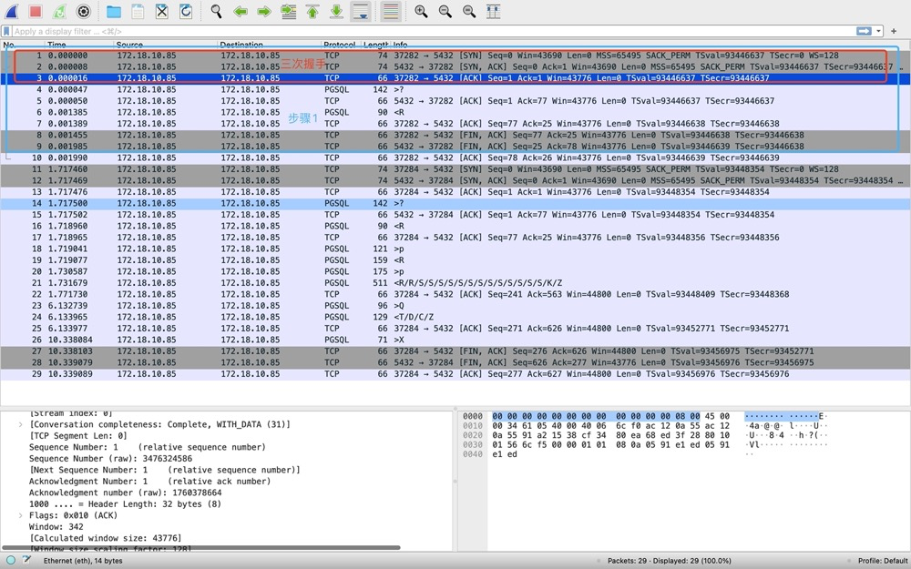
- 37282->5432 sends SYN, seq=0
- 5432->37282 sends SYN+ACK, seq=0 ack=1
- 37282->5432 sends ACK, seq=1 ack=1
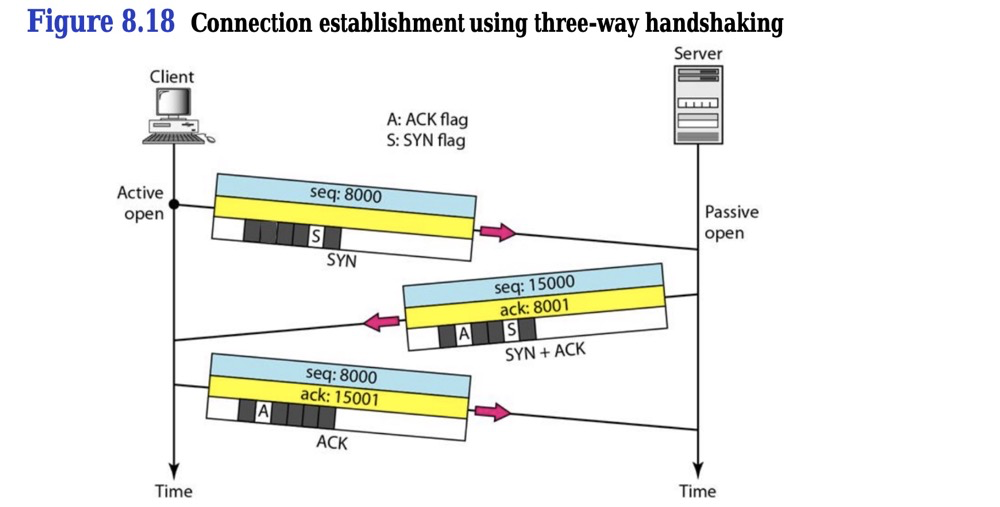
(https://www.researchgate.net/publication/340247809_Computer_Network_Chapter_8_Transport_Layer_UDP_and_TCP)
- Step 1 - Connection Request [1-10] — PGSQL protocol startup and authentication request [4-7]:
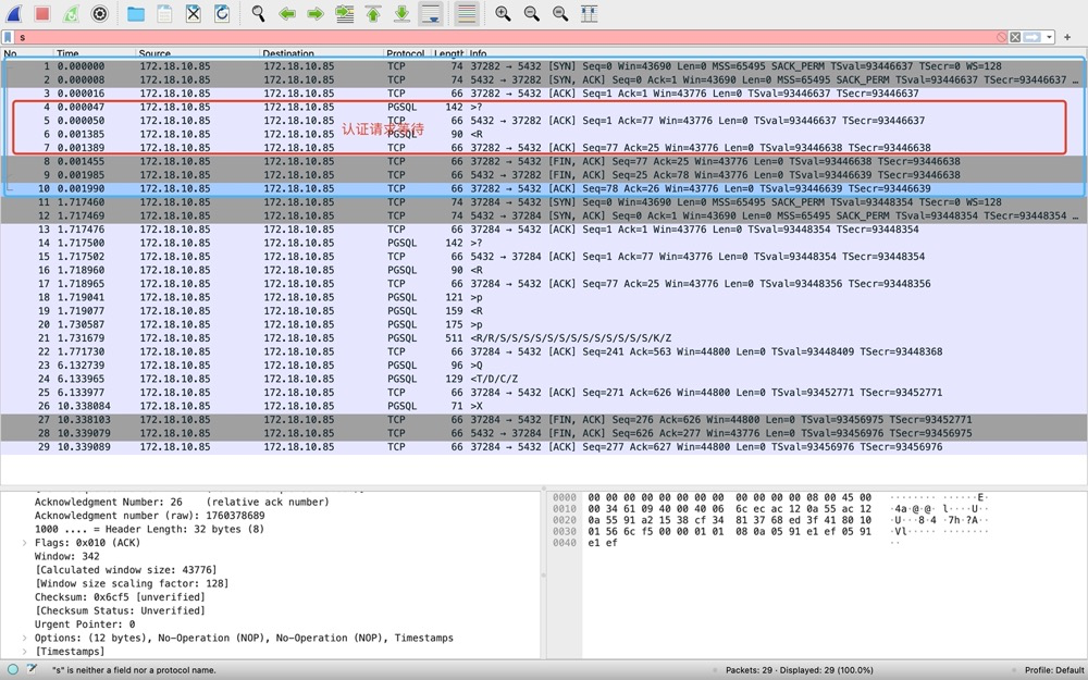
After the three-way handshake, PSQL client immediately sends a PGSQL protocol startup message to PG server [4], info: >?, the protocol startup message.
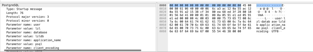
The above >? packet is 37282->5432. You don’t need to check source/destination in Transmission Control Protocol. PGSQL protocol shows even less info than TCP, but it has direction: > means 37282->5432, < means 37282<-5432.
Next PGSQL protocol message is authentication request [6], info: <R, 37282<-5432.
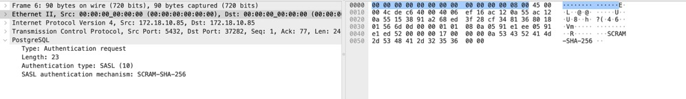
- Step 1 - Connection Request [1-10] — Three-way FIN [8-10]. After server sends PGSQL authentication request to client, client requests TCP disconnect, 3 TCP FINs (not 4; explained below). Note: at this point psql command line is waiting for password input…
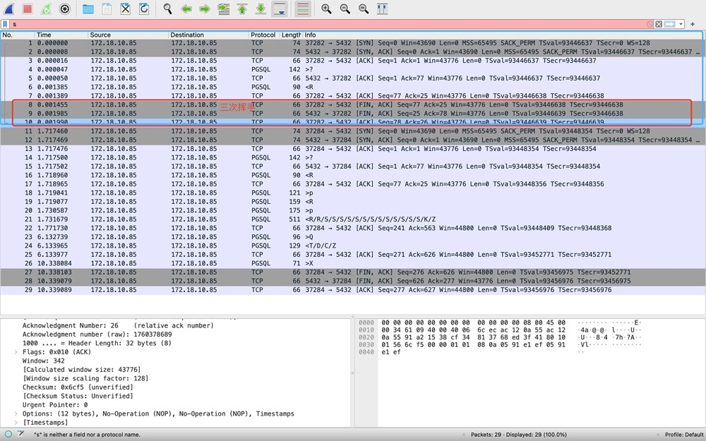
- Step 2 - Password Entry [11-22] — Three-way handshake [11-13]. Because the first TCP connection ended, establishing a connection again starts from TCP… so another three-way handshake:
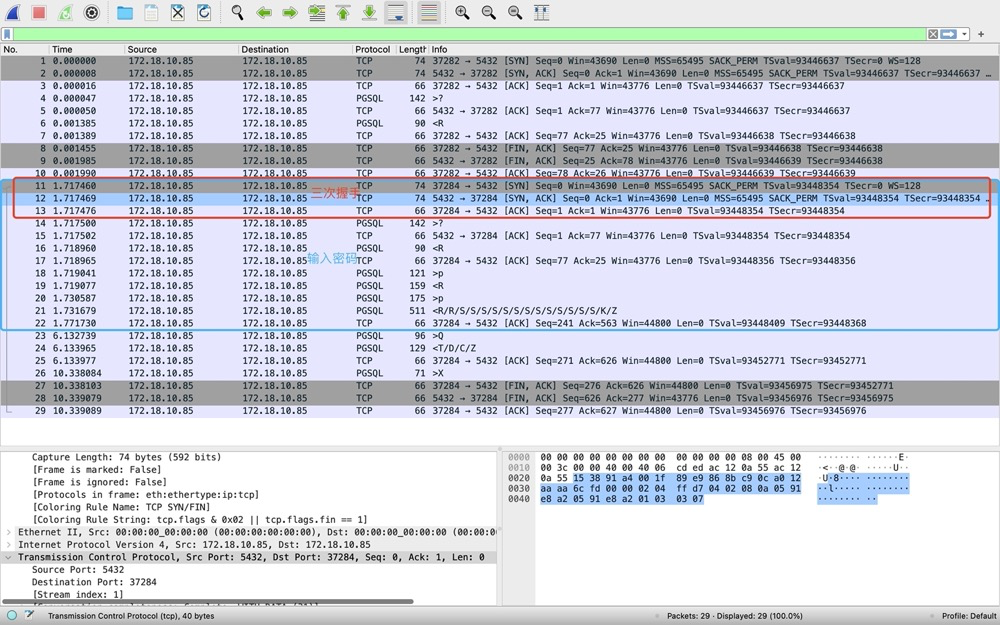
- Step 2 - Password Entry [11-22] — Password authentication [14-22]. Authentication phase is slightly more complex. [14-16] essentially does the same as [4-7] in step 1: client requests PGSQL protocol startup, server returns authentication request. Then [18-20] performs password authentication using SCRAM-SHA-256 mechanism; password authentication actually transmits 4 packets, including [21]’s two R authentication messages. Then [21] connection established: first two R’s are authentication complete; many S’s represent Parameter status: application name, charset, timezone, etc.; K represents Backend key, returning forked backend PID; Z represents ready for query.
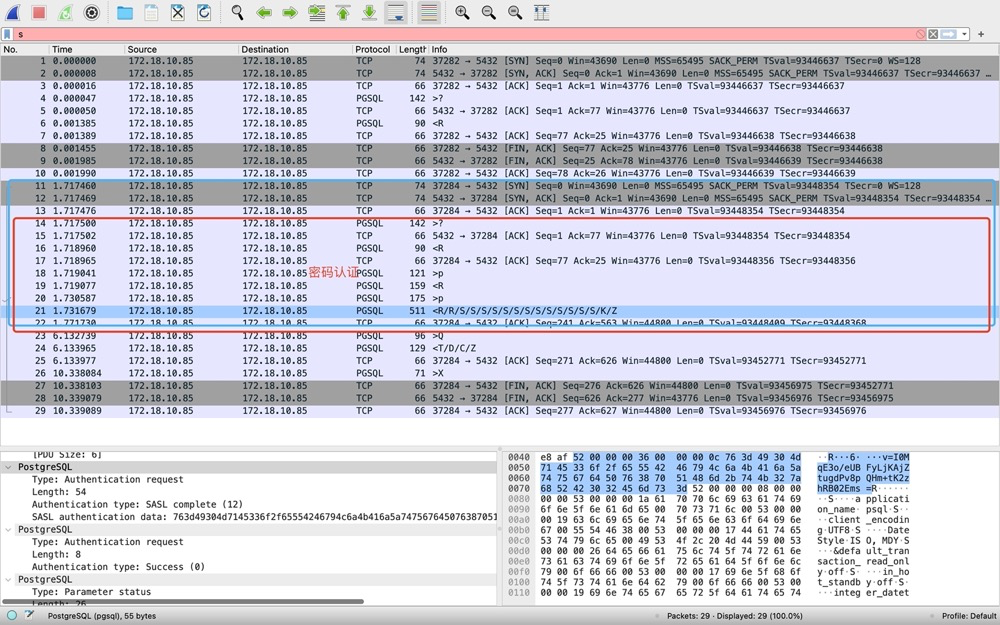
- Step 3 - SQL Query [23-25]
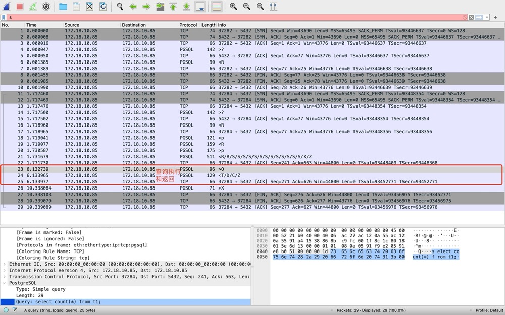
[23] Q clearly represents Query, client sends packet containing SQL; [24] returns results: T represents Row Description (here only column name “count”); D represents data row, the count result is 4, data is plaintext unencrypted:
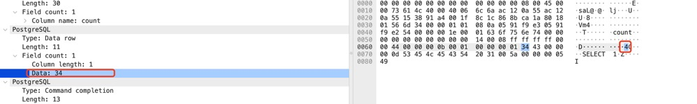
C represents Command complete; Z represents ready.
- Step 4 - Disconnect [26-29]. [26] client actively sends session end message, PGSQL protocol (corresponds to \q); [27-29] again 3 TCP FINs.
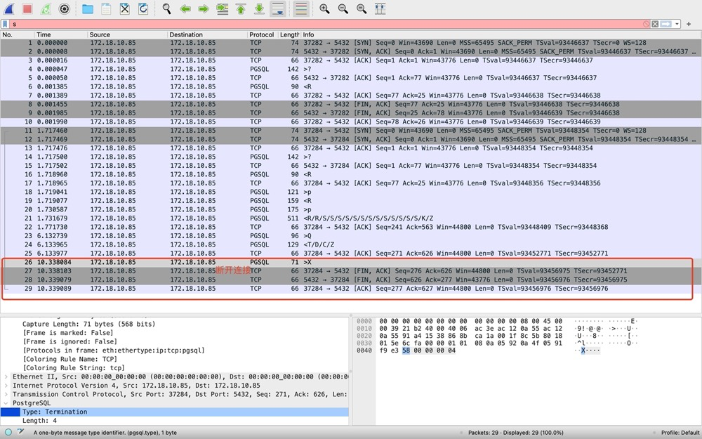
Why three FINs instead of four?
“No more data to send” AND “TCP delayed ACK mechanism enabled” means the second and third FINs merge, resulting in three FINs:
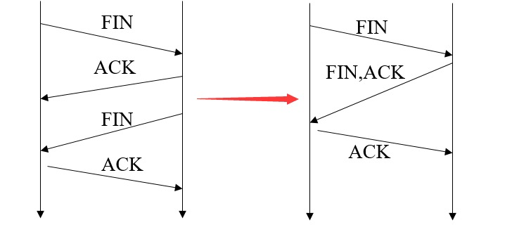
Since TCP delayed ACK is enabled by default, three-FIN scenarios appear more often than four-FIN in captures.
OK, simple PG packet capture and analysis complete. Summary network transmission diagram for this session:
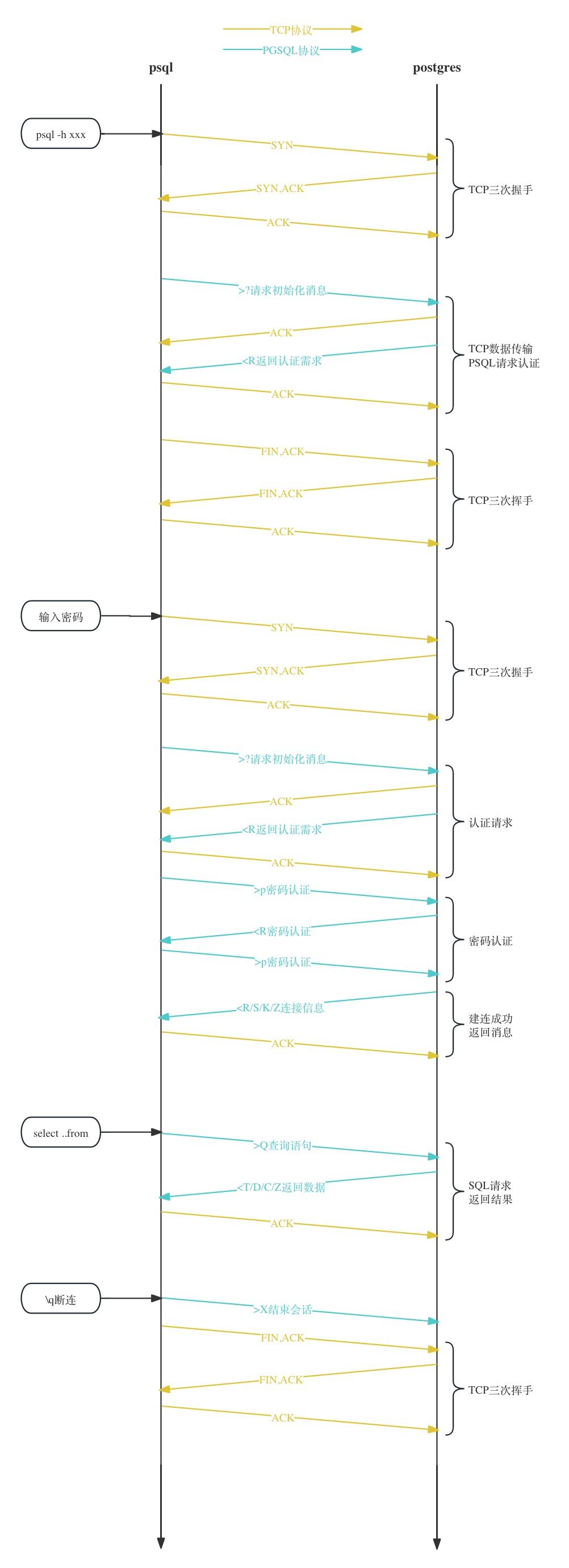
Packet capture analysis notes:
- First understand the link; typically many nodes exist between application clients and database servers: network switches, request forwarding services, etc.
- Capture on both ends simultaneously when possible
- Pay attention to capture timing and set appropriate filters
Possible packet loss points:
https://mp.weixin.qq.com/s/dF4juaW-ttI0Zn1j0z6tag
Packet loss involves NICs, drivers, and kernel protocol stack — each layer can lose packets:
- Between two VM connections, transmission failures may occur: network congestion, line errors, etc.
- After NIC receives packets, the ring buffer may overflow and drop packets
- At IP layer: routing failures, packet size exceeding MTU, etc.
- At transport layer: port not listening, resource usage exceeding kernel limits, etc.
- At socket layer: socket buffer overflow and packet loss
- At application layer: application exceptions causing packet loss
References:
38. Storage: SAN / NAS / DAS#
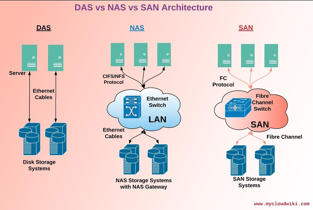
39. Lifecycle of an IO Request#
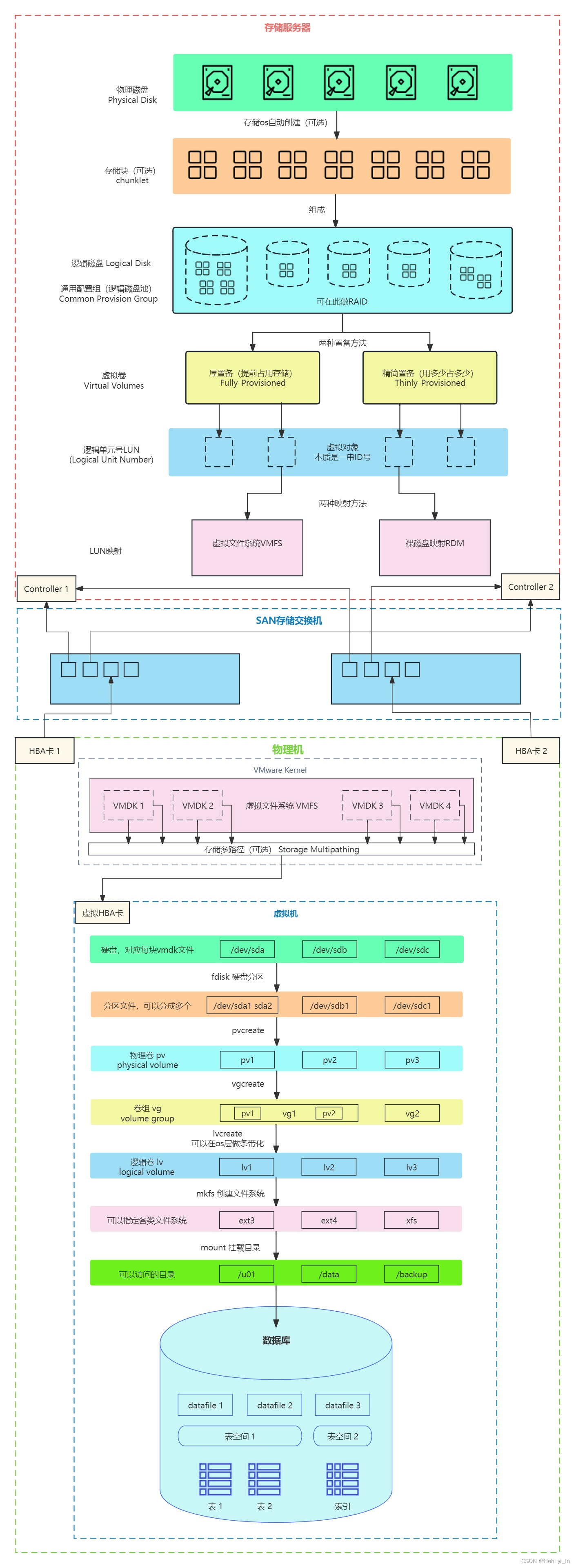
(https://blog.csdn.net/Hehuyi_In/article/details/100715177?spm=1001.2014.3001.5501)